TDII MDM (v2) (PDF)

MOMENT DISTRIBUTION METHOD
Various Methods of Application
by Cliff Leung
In this set of notes, three methods of applying the moment distribution method are
presented:
Method 1 – Release one joint in each iteration step. Unmodified stiffness factors are
used. (The original method)
Method 2 – Release multiple joints in each iteration step.
factors are used.

Unmodified stiffness

Method 3 – Release multiple joints in each iteration step. Modified stiffness factors
are used.
The moment distribution method essentially involves four steps to find the end
moments of all members:
1. Find fixed end moments (FEM)
2. Find stiffness factors (K)
3. Find distribution factors (DF)
4. Proceed with the distribution or iteration process.
Before proceeding to the example problem, let's take a look at the difference between
the unmodified and modified stiffness factors.
Unmodified and modified stiffness factors
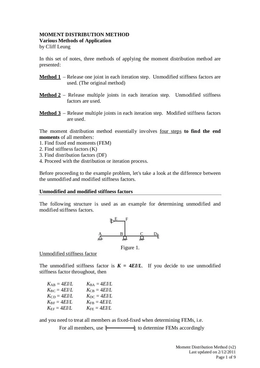
The following structure is used as an example for determining unmodified and
modified stiffness factors.
E

A

F
B

C

D

Figure 1.
Unmodified stiffness factor
The unmodified stiffness factor is K = 4EI/L. If you decide to use unmodified
stiffness factor throughout, then
KAB = 4EI/L
KBC = 4EI/L
KCD = 4EI/L
KBF = 4EI/L
KEF = 4EI/L

KBA = 4EI/L
KCB = 4EI/L
KDC = 4EI/L
KFB = 4EI/L
KFE = 4EI/L

and you need to treat all members as fixed-fixed when determining FEMs, i.e.
For all members, use
to determine FEMs accordingly

Moment Distribution Method (v2)
Last updated on 2/12/2011
Page 1 of 9

Modified stiffness factor
There are several types of modification to the stiffness factor. This set of notes
presents one of the most commonly used modifications as follows.
The modification applies to member that has one of its ends being an absolute end
of structure. What are the absolute ends in the structure above? Ans: Joint A, Joint D
and Joint E. Note that Joint F is not an absolute end.
The modified stiffness factor for this type of member is K = 3EI/L and the application
is as follows:
Use unmodified K, i.e. K = 4EI/L, for far end that is not an absolute end (or far
end fixed)
Use modified K,

i.e. K = 3EI/L, for far end that is an absolute end (or far end
pinned/roller supported)

What does far end mean? For example,
i

j

If you are finding Kij, then j is the far end
If you are finding Kji, then i is the far end

In other words, the second letter of the subscript of K indicates the far end joint.
Let’s consider the structure in Figure 1 and determine the stiffness factors with
modifications considered.
Is far end the Is the absolute far end
Stiffness factor Far end is
∴K=
absolute end?
pinned or roller
supported?
KAB
B
No
4EI/L
KBA
A
Yes
Yes
3EI/L
KBC
C
No
4EI/L
KCB
B
No
4EI/L
KCD
D
Yes
No
4EI/L
KDC
C
No
4EI/L
KBF
F
No
4EI/L
KFB
B
No
4EI/L
KEF
F
No
4EI/L
KFE
E
Yes
Yes
3EI/L
You need to treat the members which modified stiffness factor is used as fixed-pinned
when determining FEMs. ie.,
For Members AB and EF, use
For Members BC, CD and BF use

Moment Distribution Method (v2)
Last updated on 2/12/2011
Page 2 of 9

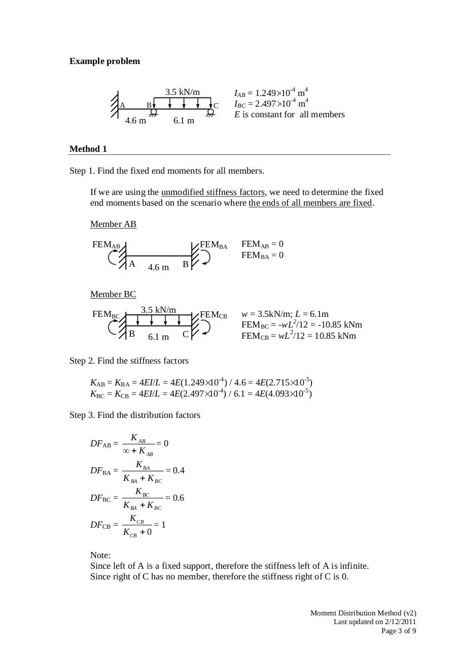
Example problem
3.5 kN/m
A

B

4.6 m

C

6.1 m

IAB = 1.249×10-4 m4
IBC = 2.497×10-4 m4
E is constant for all members

Method 1
Step 1. Find the fixed end moments for all members.
If we are using the unmodified stiffness factors, we need to determine the fixed
end moments based on the scenario where the ends of all members are fixed.
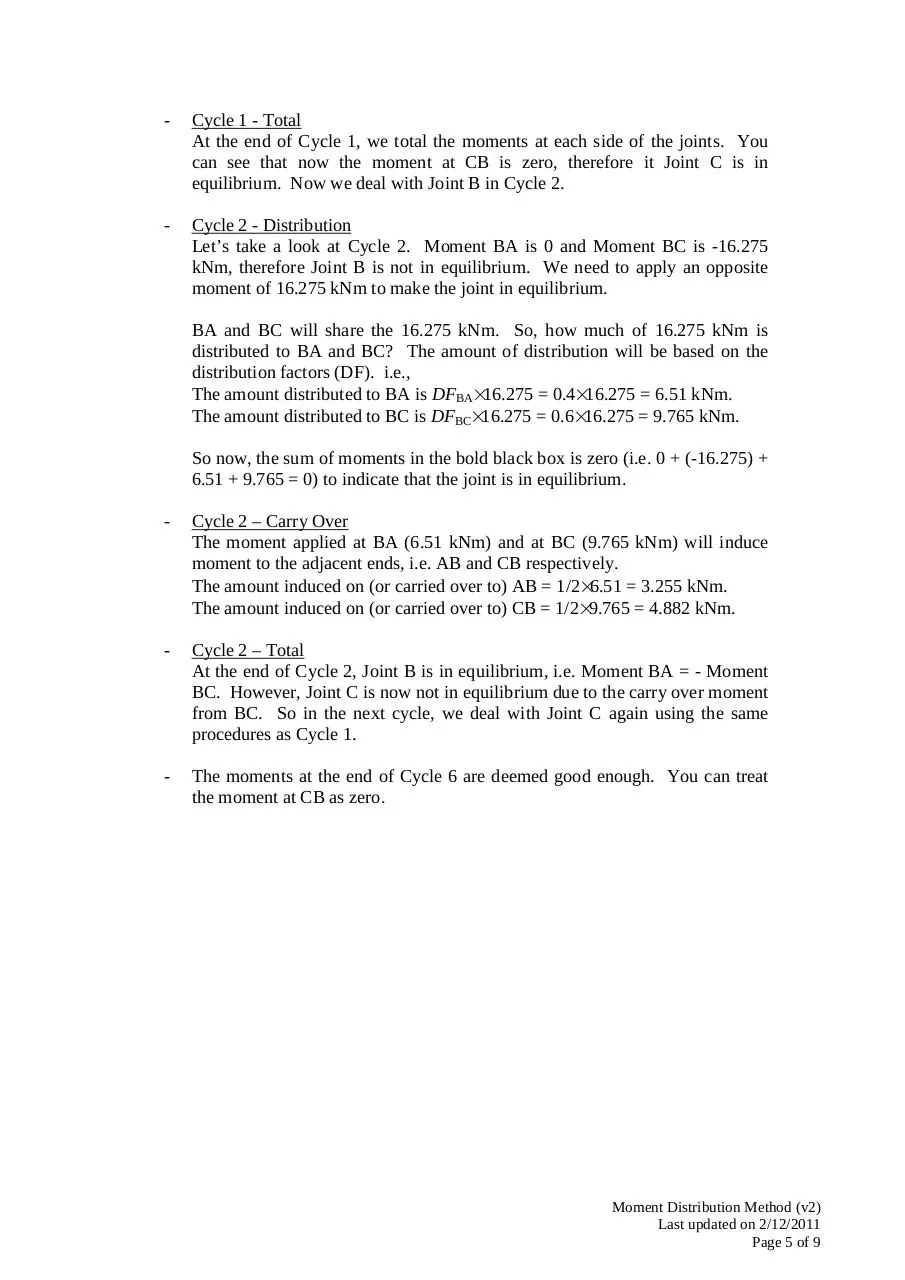
Member AB
FEMAB
A

4.6 m

FEMBA

FEMAB = 0
FEMBA = 0

FEMCB

w = 3.5kN/m; L = 6.1m
FEMBC = -wL2/12 = -10.85 kNm
FEMCB = wL2/12 = 10.85 kNm

B

Member BC
3.5 kN/m

FEMBC
B

6.1 m

C

Step 2. Find the stiffness factors
KAB = KBA = 4EI/L = 4E(1.249×10-4) / 4.6 = 4E(2.715×10-5)
KBC = KCB = 4EI/L = 4E(2.497×10-4) / 6.1 = 4E(4.093×10-5)
Step 3. Find the distribution factors

K AB
=0
∞ + K AB
K BA
= 0.4
DFBA =
K BA + K BC
K BC
DFBC =
= 0.6
K BA + K BC
K CB
DFCB =
=1
K CB + 0
DFAB =

Note:
Since left of A is a fixed support, therefore the stiffness left of A is infinite.
Since right of C has no member, therefore the stiffness right of C is 0.

Moment Distribution Method (v2)
Last updated on 2/12/2011
Page 3 of 9

Step 4. Distribution process

Cycle
1

2

3

4

5

6

Joint
DF
FEM
Dist.
CO
Total
Dist.
CO
Total
Dist.
CO
Total
Dist.
CO
Total
Dist.
CO
Total
Dist.
CO
Total

A
AB
0
0
0
0
0
0
3.255
3.255
0
0
3.255
0
0.488
3.743
0
0
3.743
0
0.073
3.816

B
BA
0.4
0
0
0
0
6.51
0
6.51
0
0
6.51
0.976
0
7.486
0
0
7.486
0.146
0
7.632

BC
0.6
-10.85
0
-5.425
-16.275
9.765
0
-6.51
0
-2.44
-8.95
1.464
0
-7.486
0
-0.366
-7.852
0.220
0
-7.632

C
CB
1
10.85
-10.85
0
0
0
4.882
4.882
-4.882
0
0
0
0.732
0.732
-0.732
0
0
0
0.110
0.11

Remarks

Unlock Joint C to make
Joint C in equilibrium
Unlock Joint B to make
Joint B in equilibrium
Unlock Joint C to make
Joint C in equilibrium
Unlock Joint B to make
Joint B in equilibrium
Unlock Joint C to make
Joint C in equilibrium
Unlock Joint B to make
Joint B in equilibrium

Good enough

Here are some explanations on the distribution process:
- In this method, we are unlocking each joint one at a time to make the joint in
equilibrium.
-

At each distribution step (i.e. Dist.), we need to apply an opposite moment to
make the unlocked joint in equilibrium. If you look at the table above, we are
trying to make the sum of all moments in the bold black box zero.

-

Cycle 1 - Distribution
Let’s take a look at Cycle 1. Since Joint C is a roller, the moment for CB
should be zero but there is currently a moment of 10.85 kNm. Therefore, we
need to apply an opposite moment of -10.85 kNm to make it in equilibrium.
So now, the numbers in the bold black box is zero (i.e. 10.85 + (-10.85) = 0).

-

Cycle 1 - Carry Over
After applying the moment of -10.85 kNm at CB, that moment applied will
induce moment to the other end of the member (i.e. BC). How much will it
induce? It will induce 1/2 of the applied moment at CB. This 1/2 is known as
the carry-over (CO) factor. The arrow indicates that 1/2 of 10.85 kNm at CB
is carried over to BC.

Moment Distribution Method (v2)
Last updated on 2/12/2011
Page 4 of 9

-

Cycle 1 - Total
At the end of Cycle 1, we total the moments at each side of the joints. You
can see that now the moment at CB is zero, therefore it Joint C is in
equilibrium. Now we deal with Joint B in Cycle 2.

-

Cycle 2 - Distribution
Let’s take a look at Cycle 2. Moment BA is 0 and Moment BC is -16.275
kNm, therefore Joint B is not in equilibrium. We need to apply an opposite
moment of 16.275 kNm to make the joint in equilibrium.
BA and BC will share the 16.275 kNm. So, how much of 16.275 kNm is
distributed to BA and BC? The amount of distribution will be based on the
distribution factors (DF). i.e.,
The amount distributed to BA is DFBA×16.275 = 0.4×16.275 = 6.51 kNm.
The amount distributed to BC is DFBC×16.275 = 0.6×16.275 = 9.765 kNm.
So now, the sum of moments in the bold black box is zero (i.e. 0 + (-16.275) +
6.51 + 9.765 = 0) to indicate that the joint is in equilibrium.

-

Cycle 2 – Carry Over
The moment applied at BA (6.51 kNm) and at BC (9.765 kNm) will induce
moment to the adjacent ends, i.e. AB and CB respectively.
The amount induced on (or carried over to) AB = 1/2×6.51 = 3.255 kNm.
The amount induced on (or carried over to) CB = 1/2×9.765 = 4.882 kNm.

-

Cycle 2 – Total
At the end of Cycle 2, Joint B is in equilibrium, i.e. Moment BA = - Moment
BC. However, Joint C is now not in equilibrium due to the carry over moment
from BC. So in the next cycle, we deal with Joint C again using the same
procedures as Cycle 1.

-

The moments at the end of Cycle 6 are deemed good enough. You can treat
the moment at CB as zero.

Moment Distribution Method (v2)
Last updated on 2/12/2011
Page 5 of 9

Method 2
In Method 1, we unlock one joint in each cycle to make that joint in equilibrium. In
Method 2, we will look at unlocking multiple joints that are not in equilibrium in each
cycle to expedite the iteration process.
Step 1. FEMs – same as Method 1
Step 2. Stiffness factors – same as Method 1
Step 3. Distribution factors – same as Method 1
Step 4. Distribution process

Cycle

1
2
3
4
5

Joint
DF
FEM
Dist.
CO
Dist.
CO
Dist.
CO
Dist.
CO
Dist.
CO
Total

A
AB
0
0
0
2.170
0
1.085
0
0.326
0
0.163
0
0.049
3.793

B
BA
0.4
0
4.34
0
2.17
0
0.651
0
0.326
0
0.098
0
7.585

BC
0.6
-10.85
6.51
-5.425
3.255
-1.628
0.977
-0.814
0.488
-0.244
0.146
-0.122
-7.707

C
CB
1
10.85
-10.85
3.255
-3.255
1.628
-1.628
0.488
-0.488
0.244
-0.244
0.073
0.073

Remarks

Unlock B and C
Unlock B and C
Unlock B and C
Unlock B and C
Unlock B and C

Good enough

Here are some explanations on the distribution process:
-

In this method, we do not need to total the moments at each side of the joints
after each cycle as in Method 1.

-

Instead, we apply an opposite moment in each Dist. step to counter the carry
over moment. In other words, after CO is done, we apply a moment opposite
to the total moment due to CO at each joint and distribute that opposite
moment to each side of the joint.
For example, at the end of Cycle 1, the total moment at Joint B after CO is 0 +
(-5.425) = -5.425 kNm. Therefore, we apply an opposite moment of 5.425
kNm to make the joint in equilibrium. This moment of 5.425 kNm is
distributed to BA and BC in the Dist. step of Cycle 2 so that Moment BA is
2.17 kNm and Moment BC is 3.255 kNm.

-

At the end, the moments calculated are similar to those obtained in Method 1.
Note that the moment-distribution method is an approximate method only and
the more iteration you perform the more accurate the results you should get.

Moment Distribution Method (v2)
Last updated on 2/12/2011
Page 6 of 9

Method3
In Method 1 and 2, we use the unmodified stiffness factors throughout our calculation.
In this method, we will try using the modified stiffness factors so as to further
expedite the iteration process.
Here are several points that you need to note when using the modified stiffness factor
that is presented in this set of notes (i.e. K=3EI/L):
1. The modified stiffness factor can be used when a member has one of its ends
an absolute end of the structure.
2. When the modified stiffness factor is used for a particular member, the member
must be treated as fixed-pinned when determining the FEMs.
3. Moment does not need to be carried over to the pinned end (absolute end) of
a member for which modified stiffness factor is used.
Step 1. Find the fixed end moments for all members.

Member AB
FEMAB

FEMBA
A

4.6 m

FEMAB = 0
FEMBA = 0

B

Member BC
3.5 kN/m

FEMBC
B

6.1 m

FEMCB
C

w = 3.5kN/m; L = 6.1m
FEMBC = -wL2/8 = -16.28 kNm
FEMCB = 0

Notice that the FEMs of Member BC in this case is different from that in
Method 1.
Step 2. Find the stiffness factors
Member AB
KAB = KBA = 4EI/L = 4E(1.249×10-4) / 4.6 = 1.086×10-4E
Member BC
Since Member BC has one of its ends (i.e. C) an absolute end of the structure,
therefore, we can use modified stiffness factor for this member.
KBC = 3EI/L = 3E(2.497×10-4) / 6.1 = 1.228×10-4E
KCB = 4EI/L = 4E(2.497×10-4) / 6.1 = 1.637×10-4E

Moment Distribution Method (v2)
Last updated on 2/12/2011
Page 7 of 9

Step 3. Find the distribution factors

K AB
=0
∞ + K AB
K BA
DFBA =
= 0.47
K BA + K BC
K BC
DFBC =
= 0.53
K BA + K BC
K CB
DFCB =
=1
K CB + 0

DFAB =

Step 4. Distribution process

Cycle

1

Joint
DF
FEM
Dist.
CO
Total

A
AB
0
0
0
3.826
3.826

B
BA
0.47
0
7.652
0
7.652

C
CB
1
0
0
0
0

BC
0.53
-16.28
8.628
0
-7.652

Remarks

Unlock B and C

Here are some notes on the distribution process:
- Note that in the distribution process, you do not need to carry the moment
from BC over to CB unlike in Methods 1 and 2, since by using the modified
stiffness factor, it has already implied that moment will not be carried over to
the pinned end.
- After Cycle 1, all joints are in equilibrium and therefore the solution is found in
just one Cycle. Comparing to Methods 1 and 2, this method of using the
modified stiffness factors can yield the solution quicker.

Bending Moment and Shear Force Diagrams
After determining the end moments using either Methods 1, 2 or 3, the question
usually asks you to draw the bending moment and shear force diagrams. To do so,
you need to determine the end forces of all members first.
3.5 kN/m
MBC
MAB
MBA
MCB
A
VAB

4.6 m

B
VBA

B

6.1 m

VBC

C
VCB

From the results of the moment distribution:
MAB = 3.256 kNm; MBA = 7.652 kNm; MBC = -7.652 kNm; MCB = 0.

Moment Distribution Method (v2)
Last updated on 2/12/2011
Page 8 of 9

Determine VAB and VBA by say ΣMA=0 and ΣV=0 for Member BA
Determine VBC and VCB by say ΣMB=0 and ΣV=0 for Member BC
Therefore, VAB = -2.371 kN; VBA = 2.371 kN; VBC = 11.93; and VCB = 9.42 kN.
The shear force and bending moment diagrams of each member are
11.93
A
-

-2.371
-2.371

B

B +

C
3.41m

12.67
+

+
-

-7.652

SFD

-9.42
BMD

-7.652

Moment Distribution Method (v2)
Last updated on 2/12/2011
Page 9 of 9