Climate shift hypothesis (PDF)

Hypothesis about mechanics of global warming from 1900 till now.
Belolipetsky P.V. 1,2 *, Bartsev S.I.2
1

Institute of computational modelling, SB RAS, Krasnoyarsk, Russia

2

Institute of biophysics, SB RAS, Krasnoyarsk, Russia

*

email: pbel@icm.krasn.ru

Abstract
We performed linear multivariate regression analysis using available estimates of natural and
anthropogenic influences and the observed surface temperature records from 1900 to 2012. We
considered four parts of Earth surface - tropics (30S-30N), northern middle altitudes (30N-60N),
Arctic (60N-75N) and southern altitudes (60S-30S). For each part (except southern altitudes) we
developed very simple linear regression models representing temperature dynamics without
continuous anthropogenic influence. The monthly average tropical SST temperature anomaly
dynamic could be adequately reproduced by only three factors - ENSO variability (Nino 3.4 index),
volcanic aerosols in stratosphere and two climate shifts in 1925/1926 and 1987/1988 years. Nothern
middle altitudes SST temperature anomaly could be reproduced in general by the same factors,
except ENSO which is changed on Pacific decadal oscillation (PDO) here. Continents in these parts
have the same dynamic but with much more variability. Arctic temperature anomalies have in
general the same dynamic as SST temperature anomalies of Atlantic ocean in northern middle
altitudes (30N-60N). We didn't manage to build any adequate regression model for southern
altitudes with or without anthropogenic influences, but it doesn't look like temperatures here are
determined by continuous anthropogenic influence. The results enable us to suggest a quantitive
hypothesis alternative to IPCC view about a mechanic of observed in past century climate change.
1. Introduction
The prime indicator of global warming is, by definition, global mean temperature. The 20 th
century increase in global mean temperature has been well documented – there was an increase of

about 0.75 °C between 1880 and 2008 (Intergovernmental Panel on Climate Change (IPCC) 2007).
Both natural and anthropogenic influences have caused twentieth century climate change but their
relative roles and regional impacts are still under debate (Lean and Rind 2008). Studies based on
atmosphere-ocean general circulation models (AOGCMs) conclude that increasing anthropogenic
gas concentrations (greenhouse gases (GHGs) and tropospheric aerosols) produced 0.3–0.5 °C per
century warming over the 1906–1996 period and were the dominant cause of global surface
warming after 1976 (Allen et al. 2006). However, this warming was not straightforward – global
temperature increased in the first part of the century, then slightly decreased in the years 1940-1970,
then increased again and stayed almost flat during the last decade. Additionally temperatures have
always fluctuated rapidly with amplitudes up to 0.5 °C over small time scales, e.g. years. Moreover,
AOGCMs have not been able to reproduce all of these features (IPCC 2007). Lean and Rind (2008,
2009) performed multivariate linear regression analysis of the natural and anthropogenic influences
on global surface temperature anomalies. They concluded that much of the variability in global
climate arises from processes that can be identified and their impact on the global surface
temperature quantified by direct linear association with the observations. And they were able to
reconstruct the observed temperature anomalies only by associating the surface warming with
anthropogenic forcing.
We investigated the possibility of reconstruction the observed temperature anomalies without
anthropogenic forcing by means of regression analysis. Eventually we found that it is possible to
reconstruct adequately observed temperature anomalies with two climate regime shifts in 1925/1926
and in 1987/1988 years instead of continuous anthropogenic forcing. The reality of these shifts and
details highlighting their influence are described later.

2. Analysis and datasets
Most of the used datasets are freely available at Climate Explorer site (climexp.knmi.nl).
And all the calculations were made in Excel by means of standard functions. A reconstruction of
monthly mean surface temperature anomalies, TR , from input parameters is performed by:
n

T ( t ) = c o + ∑ c i ⋅ X i ( t − ∆t i ) ,

(1)

i =1

Here X i are determining climate factors; ∆t i are the lags in months; ci - the fitted coefficients and
n – the number of harmonics in regression. The fitted coefficients are obtained by standard Excel
function for multivariate linear regression.
In presented analysis we used several reconstructions of observed temperature anomalies HadSST2, Reynolds v2, HadCRUT4 and NCDC datasets. For the period from 1900 till the
beginning of 1980s we used HadSST2 and later Reynolds v2 as SST anomalies (as we thought that
remote sensing data is more precise). Then we need to analyze land areas or combined land and
ocean areas we used HadCRUT4. And as there were big spaces in southern altitudes HadCRUT4
time series we used NCDC reconstruction for this area (30S-90S). Anthropogenic influence,
volcanic aerosols, ENSO and Pacific decadal oscillation were considered as factors determining
observed temperature anomalies. Volcanic aerosols in the stratosphere were compiled by Sato et al.
(1993) from records kept since 1850 and updated from climexp.knmi.nl till now. Warming
greenhouse gases were considered as a proxy for the anthropogenic forcing as the other components
(land use, snow albedo changes and tropospheric aerosols) are very uncertain. We used the same
anthropogenic

greenhouse

gases

forcing

as

in

GISS

global

climate

models

(http://data.giss.nasa.gov/modelforce/Fe.1880-2011.txt) with 10 year lag (the same as in Lean and
Rind (2008)). As a proxy for ENSO we considered Nino34 index obtained from HadISST1. And for
the PDO we used reconstruction from ERSST. All used datasets except anthropogenic greenhouse
gases forcing were prepared and downloaded from Climate Explorer site.

3. Tropical belt (30S-30N)
Let's consider tropics (30S-30N), northern middle altitudes (30N-60N), Arctic (60N-75N)
and southern altitudes (60S-30S) separately. At first we will consider tropical SST (Fig. 1). Most of
variability here is explained by ENSO. Also the forcing of volcanic eruptions is clearly seen. And
from first view these natural forcing should be accompanied by some continuous warming, which
can be attributed to anthropogenic greenhouse gases. In this case tropical SST anomalies could be
adequately reconstructed by linear regression with appropriate lags - one month for ENSO and four
months for volcanic aerosols (Fig. 1).

0.9
0.7
0.5
0.3
0.1
-0.1
-0.3
-0.5
-0.7
-0.9
1900

1910

1920

1930

1940

1950

1960

1970

1980

1990

2000

2010

Fig. 1. Blue line - observations of SST anomalies in tropics, red line - linear regression model with anthropogenic
forcing. Correlation coefficient 0.86.

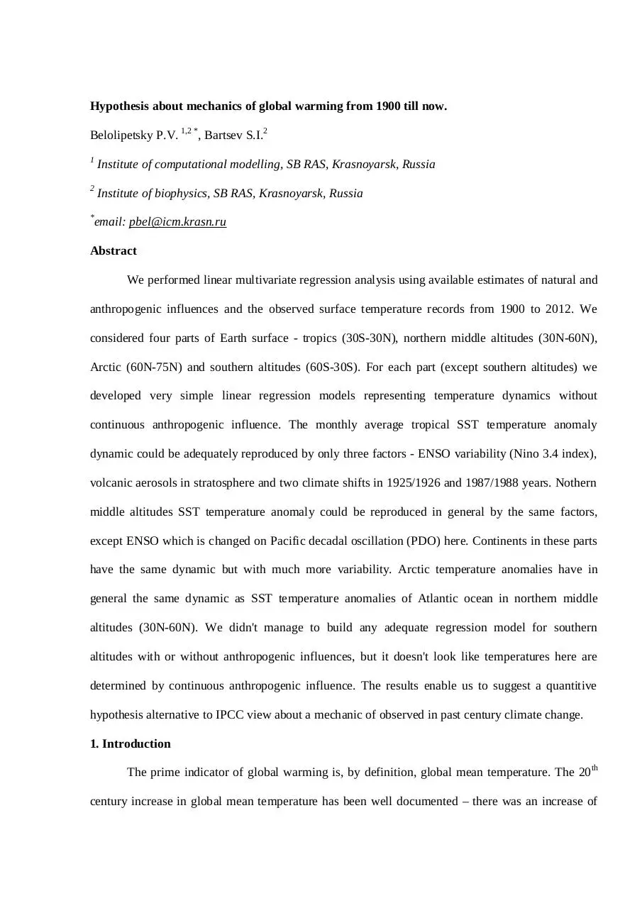
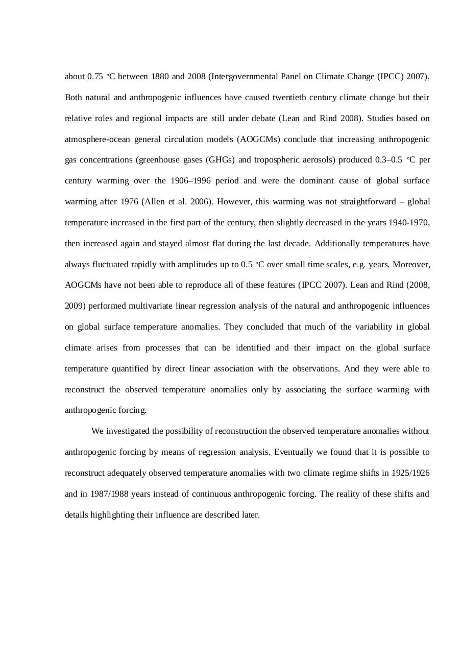
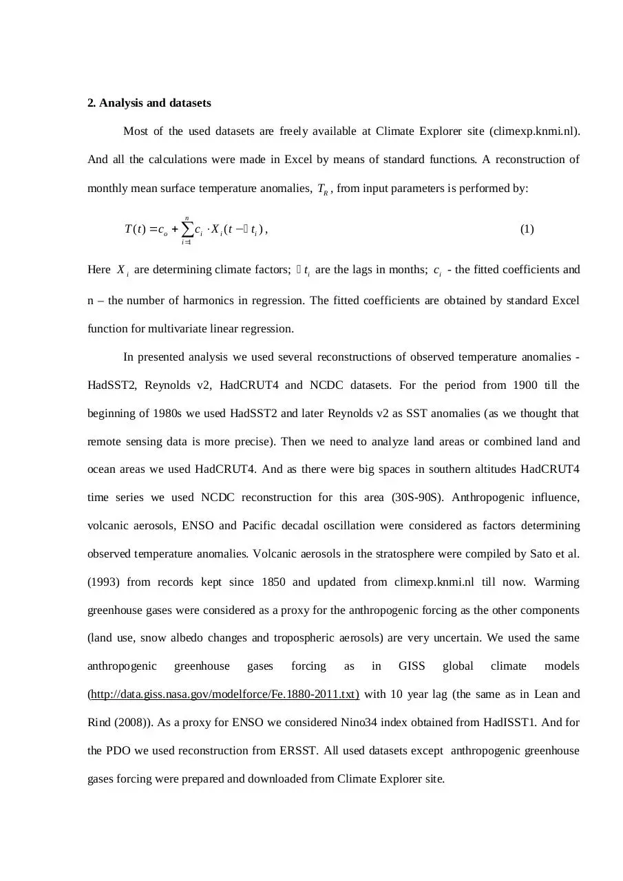
But it is possible to notice that linear regression without anthropogenic forcing reproduce
quite well anomalies from middle 80th till now (Fig. 2), but fails to reproduce previous period with
obtained coefficients. From the other side regression by ENSO and volcanic aerosols reproduce
period from 1950 till middle 80th (Fig. 3), but inadequate later. This suggests that there may be a
climate regime shift somewhere in the middle 80th. So we added another determining climate factor
- climate regime index, a step function witch equals zero before shift and equals one after. In this
case temperature anomalies reproduced without anthropogenic forcing at least from 1950s (Fig. 4).

0.7
0.5
0.3
0.1
-0.1
-0.3
-0.5
-0.7
-0.9
1900

1910

1920

1930

1940

1950

1960

1970

1980

1990

2000

2010

Fig. 2. Blue line - SST in tropics, red line - regression without anthropogenic forcing, studied by 1984-2010 years.

0.7
0.5
0.3
0.1
-0.1
-0.3
-0.5
-0.7
-0.9
1900

1910

1920

1930

1940

1950

1960

1970

1980

1990

2000

2010

Fig. 3. Blue line - SST in tropics, red line - regression without anthropogenic forcing, studied by 1950-1980 years.

0.9
0.7
0.5
0.3
0.1
-0.1
-0.3
-0.5
-0.7
-0.9
1900

1910

1920

1930

1940

1950

1960

1970

1980

1990

2000

2010

Fig. 4. Blue line - SST in tropics, red line - regression with shift in 1987 instead of anthropogenic forcing.

We considered different parts (Pacific, Atlantic, Indian) of tropical SST and found that
regime shift was localized in 1987. But we didn't know any climate shift in that time. So we began

to search publications about shifts in late 80th. At first we found evidence for biological or
ecological regime shifts. Shifts were observed in birds populations (Veit et. al 1996), fish
populations (Chavez et. al 2003), combined physical and biological variables (Hare and Mantua,
2000; de Young et. al 2004), local ecosystems (Tian et. al 2008) and even in global carbon cycle
(Sarmiento et. al 2010).
Then we found an articles about regime shifts in the northern hemisphere SST field
(Yasunaka and Hanawa 2002; Lo and Hsu 2010). Yasunaka and Hanawa (2002) applied an
empirical orthogonal function (EOF) analysis and detected six regime shifts in the period from
1910s to the 1990s: 1925/1926, 1945/1946, 1957/1958, 1970/1971, 1976/1977 and 1988/1989.
However our analysis shows that from 1950s temperature anomalies associated in general with
ENSO and their reproduction by linear regression doesn’t require accounting shifts of 1957/1958,
1970/1971, 1976/1977.
Possible answer exists in the work by Yasunaka and Hanawa (2002) yet. It is written:
"According to spatial pattern correlation between SST difference maps of regime shifts, it is found
that the 1945/1946, 1957/1958, 1970/1971 and 1976/1977 regime shifts are similar pattern, while
the 1925/1926 and 1988/1989 regime shifts are somewhat different." And according to this we
added another shift of the same magnitude in climate regime index between 1925 and 1926 (so step
function equals -1 before 1926, 0 between 1926 and 1987 and 1 after). In this case we obtained
adequate reconstruction from 1900 till now (Fig. 5).
Quite remarkable moment is that linear regression coefficients can be fitted by the data from
1910 till 1940 (15 years to both side from shift in 1925/1926) and quite well reproduce the whole
period from 1900 till now (Fig. 6).

0.9
0.7
0.5
0.3
0.1
-0.1
-0.3
-0.5
-0.7
-0.9
1900

1910

1920

1930

1940

1950

1960

1970

1980

1990

2000

2010

Fig. 5. Blue line - SST in tropics, red line - regression with shifts in 1925/1926 and 1987. Correlation coefficient 0.86.

0.9
0.7
0.5
0.3
0.1
-0.1
-0.3
-0.5
-0.7
-0.9
1900

1910

1920

1930

1940

1950

1960

1970

1980

1990

2000

2010

Fig. 6. Blue line - SST in tropics, red line - regression with shifts in 1925/1926 and 1987, studied by 1910-1940 years.
Correlation coefficient 0.85.

So tropical SST could be reproduced by three factors ENSO variations, volcanoes and
regime shift index. What about whole tropical belt including land areas? Temperatures over land
introduce more short term variability, which is not reproduced, but in general dynamic is
reproduced (Fig. 7). As Pacific ocean occupies near half of this area, it could happen so, that we
reproduce only Pacific anomalies. So we performed separate linear regression for different parts of
tropics - Pacific ocean, Indian ocean, Atlantic ocean and land areas. It was found that in general
linear regression reproduce anomalies for each part. Pacific ocean reproduced with near the same

quality as whole belt. Indian and especially Atlantic ocean have more variability and less correlation
with used ENSO Nino34 index.

0.9
0.7
0.5
0.3
0.1
-0.1
-0.3
-0.5
-0.7
-0.9
1900

1910

1920

1930

1940

1950

1960

1970

1980

1990

2000

2010

Fig. 7. Blue line - temperature anomalies in tropics, red line - regression. Correlation coefficient 0.86.

4. Northern altitudes (30N-90N)
We considered two parts in northern altitudes - northern middle altitudes (30N-60N) and
Arctic (60N-75N). There were only small number of temperature observations most of studied
period in polar region (75N-90N) so we omitted it. We performed the same linear regression
analysis for middle altitude SST, as for tropics. Here instead of ENSO we used Pacific decadal
oscillation index (without lag) and as in the tropics the same time series of volcanic aerosols (with
four month lag). For a good reconstruction in this region climate shifts should happened later than in
the tropics - in the middle of 1926 instead of 1925/1926 boundary and in the first part of 1988
instead of middle 1987. Again SST reproduced quite well (Fig. 8). And as in the tropics linear
regression coefficients can be fitted by the data from 1900 till 1940 and quite well except for
volcanic eruptions reproduce the whole period from 1900 till now (Fig. 9). If we will use
anthropogenic greenhouse gases forcing instead of climate regime index here like in fig. 1 of tropics,
reproduction of SST anomalies before 1950 is worse (Fig. 10). As in the tropics land areas introduce
more short term variability (and more than in the tropics, because land area here is bigger), but in
general observed temperature anomalies reproduced, of course except short term variability.

0.9
0.7
0.5
0.3
0.1
-0.1
-0.3
-0.5
-0.7
-0.9
1900

1910

1920

1930

1940

1950

1960

1970

1980

1990

2000

2010

Fig. 8. Blue line - northern middle altitudes SST, red line - regression with shifts in 1926 and 1988. Correlation 0.83.

0.9
0.7
0.5
0.3
0.1
-0.1
-0.3
-0.5
-0.7
-0.9
1900

1910

1920

1930

1940

1950

1960

1970

1980

1990

2000

2010

Fig. 9. Blue line - the same as in fig. 8, red line - regression with shifts in 1926 and 1988, studied by 1900-1940 years.
Correlation coefficient 0.8.

0.9
0.7
0.5
0.3
0.1
-0.1
-0.3
-0.5
-0.7
-0.9
1900

1910

1920

1930

1940

1950

1960

1970

1980

1990

2000

2010

Fig. 10. Blue line - the same as in fig. 8, red line - regression with anthropogenic GHGs forcing. Correlation 0.74.

Arctic (60N-75N) monthly temperature anomalies are highly variable. May be the reason is
small square of area mostly covered by land. So we performed regression analysis for yearly
averaged temperature anomalies. We argue that climate anomalies in this region determined mainly
by inflow of warm waters from North Atlantic. As a proxy for this factor we used North Atlantic
SST in northern middle altitudes (30N-60N, 75W-0W). Main trends of Arctic temperature
anomalies are reproduced (Fig. 11). And again remarkable moment coefficients of regression can be
fitted only by data from 1900 till 1940 with small changes in quality. As dynamic of SST anomalies
in northern middle altitudes could be reproduced without continuous anthropogenic forcing, so
Arctic temperatures also could be reproduced without it.
1.5
1
0.5
0
-0.5
-1
-1.5
-2
1900

1910

1920

1930

1940

1950

1960

1970

1980

1990

2000

2010

Fig. 11. Blue line - Arctic temperature anomalies, red line - linear regression model.

5. Southern altitudes (30S-90S)
Temperature observations are rare in this region. We think that they are especially rare in
Antarctic continent. So we considered two variants - temperature anomalies in whole region (30S90S) (Fig. 13) and in altitudes 30S-60S (Fig. 14). We weren't able to develop any adequate
regression model with or without anthropogenic forcing for the observed dynamics. But
CMIP5/IPCC climate models also didn't simulate this region properly (Fig. 13 and Fig. 14). Most
remarkable difference is near zero trend after 1980 in observations and big trend in CMIP5/IPCC
models. In general observations show warming trend in 20th century, but it not looks like forced by

anthropogenic greenhouse gases, because most of warming occurred before 1980 and after 1980
dynamic is near flat.

0.9
0.7
0.5
0.3
0.1
-0.1
-0.3
-0.5
-0.7
-0.9
1900

1910

1920

1930

1940

1950

1960

1970

1980

1990

2000

2010

Fig. 13. Blue line - observed temperature anomalies (30S-90S), green line - CMIP5/IPCC climate models mean (30S90S), red line - linear regression on two shifts.

0.9
0.7
0.5
0.3
0.1
-0.1
-0.3
-0.5
-0.7
-0.9
1900

1910

1920

1930

1940

1950

1960

1970

1980

1990

2000

2010

Fig. 14. Blue line - observed temperature anomalies (30S-60S), green line - CMIP5/IPCC climate models mean (30S60S), red line - linear regression on two shifts.

6. Summary
There is always a risk that multiple regression analysis may misattribute significance to
unrelated factors. From this point of view a number of empirical analyses were critically considered
by Benestad and Schmidt (2009). But as we look more broadly at the field the same risk exists for
all models – statistical ones, those based on simple ordinary equations, and AOGCMs. For example,

AOGCMs are based on known, well-established physical laws but they include many parameters
that are tuned during calibration and the verification process. Of course we have much more
freedom during multiple regression and have only qualitative thoughts about involved physical
mechanisms, so the presented relationships should be considered as a possible connection between
different influences and climate.
However, developed linear regression models are able to capture most of the dynamics in the
surface temperature record without continuous anthropogenic forcing. It should be highlighted that
if we concede two climate shifts in 1925/1926 and in 1987/1988 main features of observed in the
past century temperature anomalies can be very easily explained. In this case linear regression
shows that each shift change the mean values of sea surface temperatures by 0.28 °C in tropics and
by 0.36 °C in northern middle altitudes. Even if we consider these shifts separately (e.g. use two
climate regime indexes in linear regression - one with shift in 1925/1926 and another in 1987/1988)
the amplitudes will be near the same - 0.26 °C and 0.28 °C for tropics, 0.38 °C and 0.34 °C for
northern middle altitudes. From the other side there are many independent evidences that these shifts
are real phenomena (Veit et. al 1996; Chavez et. al 2003; Hare and Mantua, 2000; de Young et. al
2004; Tian et. al 2008; Sarmiento et. al 2010; Yasunaka and Hanawa 2002, Lo and Hsu 2010).
Lo and Hsu (2010) investigated extratropical Nothern Hemisphere temperature anomalies
and suggested near the same hypothesis, that the main reason of recently observed warming is
climate shift in 1987. They found unprecedented from early 1940s phenomenon in the late 1980s temperature fluctuation synchronization in widespread areas of Northern Hemisphere. Analyzing
spatial fields dynamic they concluded that this shift is a natural phenomenon and it was not
simulated by CMIP3/IPCC climate models. Their conclusions were obtained by means of quite
complicated statistical methods.
In our case by means of very simple linear regression analysis we noticed the possibility of
climate shift in 1987. Then found the evidence of similar shift in 1925/1926. (Yasunaka and Hanawa

2002). Eventually we developed simple linear regression models which are capable reproducing
main features of temperature anomalies for altitudes from 30S to 75N without continuous
anthropogenic forcing.
There are two remarkable moments. The first one is that linear regression coefficients can be
fitted by the small part of data (from 1900 till 1940 for example) and quite well reproduce the whole
period from 1900 till now. The second one is that good quality of reproduction is achieved by using
only three factors (ENSO/PDO, volcanoes and shifts for tropics/northern middle altitudes).
We are not speculating here about physical mechanisms and reasons of shifts. There are
many possible variants as climate is complex nonlinear dynamical system. The reasons may be
intrinsic causes, some indirect solar or volcanic forcing, or result of anthropogenic forcing. In each
case we argue that presented hypothesis that observed warming occurred not continuously but by
means of shift should be carefully considered.
Acknowledgments. We thank V.M. Belolipetsky and A.G. Degermendzhy for continuous support
of our investigations.
References
Allen MR et al. (2006) Quantifying anthropogenic influence on recent near-surface
temperature change. Surv. Geophys., 27, 491 – 544. doi:10.1007/s10712-006-9011-6.
Benestad RE, Schmidt GA (2009) Solar trends and global warming. J. Geophys. Res., 114,
D14101.
Chavez FP, Ryan J, Lluch-Cota SE, Miguel Niquen C (2003) From Anchovies to Sardines
and back: multidecadal change in the Pacific Ocean. Science, 299, 217-221.
deYoung B, Harris R, Alheit J, Beaugrand G, Mantua N, Shannon L (2004) Detection regime
shifts in the ocean: data considerations. Progress in oceanography, 60, 143-164.
Hare SR, Mantua NJ (2000) Empirical evidence for North Pacific regime shifts in 1977 and
1989. Progress in oceanography, 47, 103-145.

Intergovernmental Panel on Climate Change (2007) Climate Change 2007: The Physical
Science Basis, Contribution of Working Group I to the Fourth Assessment Report of the
Intergovernmental Panel on Climate Change, edited by S. Solomon et al., Cambridge Univ. Press,
Cambridge, U. K.
Lean JL, Rind DH (2008) How natural and anthropogenic influences alter global and
regional

surface

temperatures:

1889

to

2006.

Geophys.

Res.

Lett.,

35,

L18701,

doi:10.1029/2008GL034864.
Lean JL, Rind DH (2009) How will Earth’s surface temperature change in future decades?
Geophys. Res. Lett., 36, L15708.
Lo TT, Hsu HH (2010) Change in the dominant decadal patterns and the late 1980s abrupt
warming in the extratropical northern hemisphere. Atmospheric Science Letters, 11, 210–215.
Sarmiento JL, Gloor M, Gruber N, Beaulieu C, Jacobson AR, Mikaloff Fletcher SE, Pacala
S, Rodgers K (2010) Trends and regional distributions of land and ocean carbon sinks.
Biogeoscinces, 7, 2351-2367.
Sato M, Hansen JE, McCormick MP, Pollack JB (1993) Stratospheric aerosol optical depths,
1850 – 1990. J. Geophys. Res., 98, 22,987–22,994.
Tian Y, Kidokoro H, Watanabe T, Iguchi N (2008) The late 1980s regime shift in the
ecosystem of Tsushima warm current in the Japan/East Sea: Evidence from historical data and
possible mechanisms. Progress in oceanography, 77, 127-145.
Veit RR, Pyle P, McGowan JA (1996) Ocean warming and long-term change in pelagic bird
abundance within the California current system. Marine ecology progress series, Vol. 139, 11-18.
Yasunaka S, Hanawa K (2002) Regime shifts found in Northern Hemisphere SST Field.
Journal of meteorological society of Japan, Vol. 80, No. 1, pp. 119-135.