Applied Statistics Dehar Hamdaoui Lecocq Sitbon (PDF)

Applied
Statistics
Sitbon Pascal
Dehar Madjer
Hamdaoui Amine
Lecocq Thomas

Machine learning
algorithms applied to
insult detection in
online forums
ENSAE Paris Tech 2013-2014

1

Sitbon Pascal

Dehar Madjer

Hamdaoui Amine

Lecocq Thomas

Applied Statistics

MACHINE LEARNING ALGORITHMS APPLIED TO INSULT
DETECTION IN ONLINE FORUMS

Contents
INTRODUCTION.........................................................................................................3

I)

OPTIMIZATION IN LEARNING ...............................................................................3
A) Descriptive statistics ............................................................................................................................... 3
B) Generalization error ............................................................................................................................... 4
C) Regularization & gradient method..................................................................................................... 5

II)

SOME WELL-KNOWN CLASSIFIERS......................................................................................... 7
A) Support Vector Machines ....................................................................................................................... 7
1) Theory ............................................................................................................................................................ 7
 Linearly separable set ................................................................................................................. 8
 Linearly inseparable set .......................................................................................................... 10
2) Simulations ................................................................................................................................................ 11
 Linear kernel function .............................................................................................................. 11
 Radial basis kernel function ................................................................................................... 11
B) Decision trees ......................................................................................................................................... 15
1) Theory ......................................................................................................................................................... 15
2) Simulations ................................................................................................................................................ 17
C) Logistic regression ................................................................................................................................ 17
1) Theory ......................................................................................................................................................... 17
2) Simulations ................................................................................................................................................ 20

III)

ENSEMBLE METHODS ........................................................................................... 24
A) Forests of randomized trees................................................................................................................. 24
 Random Forests ...................................................................................................................................... 24
 Extremely Randomized Trees........................................................................................................... 25
B) AdaBoost...................................................................................................................................................... 28
 AdaBoost with SVM-based component classifiers ................................................................... 28
 AdaBoost with Decision Tree based component classifiers ................................................. 29

CONCLUSION ............................................................................................................ 30

2

Sitbon Pascal

Dehar Madjer

Hamdaoui Amine

Lecocq Thomas

Applied Statistics

MACHINE LEARNING ALGORITHMS APPLIED TO INSULT
DETECTION IN ONLINE FORUMS

INTRODUCTION
Machine learning is a branch of artificial intelligence about constructing and studying systems that can
learn from data. In 1959, Arthur Samuel, a famous pioneer in the field of artificial intelligence and computer
science, gave a formal and interesting definition of machine learning: “A computer program is said to learn
from experience E with respect to some class of tasks T and performance measure P, if its performance at tasks
in T, as measured by P, improves with experience E". This sentence puts the stress on the main principle of
machine learning techniques: a general inductive process automatically builds a classifier by learning, from a
set of preclassified documents (called training set), the characteristics of the categories. More precisely, our
goal is to train a machine learning system on forum messages to learn to distinguish between insulting
messages and “clean” messages. In order to study a wider range of classifiers, we decided to illustrate three
different classification methods that we discuss later. Rather than being exhaustive and presenting all kind of
classifiers, we preferred to take the time to explain all the mathematical background behind the learning
methods we chose. Indeed, one has to understand what is going on behind an algorithm if he wants to make it
better.
The outline of this document is as follows. Part 1 starts with some descriptive statistics and provides some
background on optimization, regularization which is a crucial concept in machine learning and gradient
methods which are used in several of the training methods we describe. Part 2 gives the basic theory about
three different kinds of classification methods: support vector machines, logistic regression and decision tree.
Part 3 tries to go further and to optimize the algorithms obtained in part 2.

I.

OPTIMIZATION IN LEARNING
A) Descriptive statistics

We have three different datasets for our work: a small one, a medium one and a large one. We call the
number of observations and the dimension of each observation –inputs–, then, our dataset is a matrix –called
–with rows and columns. Depending on the dataset we choose, is either 2245, or 16294, or 57509. This
diversity is interesting for comparisons and also when it comes to overfitting issues. Each column is
proportional to the number of occurrences of a word in the sentence. For instance, the first column could
represent the number of occurrences of the word “fuck” in the messages. Actually, it is not exactly the number
of occurrences since our data is normalized, nonetheless, it is proportional. This modes is called Bag-of-words.
For each of the three matrix,
, which means that the number of messages does not change from a
database to another; the changes only affect the number of columns. The training dataset is completed with a
vector
classifying every row –i.e. messages– of the matrix depending on whether it is considered as
insulting or not. To illustrate it more formally, the
value of is either 1 if the message corresponding to the
row of is considered as insulting or -1 if it is not. Therefore, we can give an analytic expression to our
training dataset:
{(⃗⃗⃗ )
{
} ⃗⃗⃗
}
⃗⃗⃗⃗ corresponds to the row of , it can be seen as a message
corresponds to the
value of , it is the label of ⃗⃗⃗
When we look closely at the repartition of our training dataset, we can see that it is imbalanced. Indeed, there
are 1742 insulting messages (26% of total messages) and then 4852 clean messages. Note that such
disequilibrium can affect the efficiency of an algorithm, we discuss it in more detail in §II.A)2)v). Note also that

3

Sitbon Pascal

Dehar Madjer

Hamdaoui Amine

Lecocq Thomas

MACHINE LEARNING ALGORITHMS APPLIED TO INSULT
DETECTION IN ONLINE FORUMS

Applied Statistics

the three matrices at our disposal are sparse matrices (a spare matrix stores only the non-zero elements of a
dense matrix) and it has several advantages:



It takes less space than dense matrices especially when there are many “0”.
It enables algorithms to be much faster since they can scan matrices and make operations quickly.

B) Generalization error
Supervised learning is the machine learning task of inferring a function from labeled training data. To
describe our problem formally, our goal is to learn a function
given a training set, so that ( ) is a
good predictor for the value of associated to (Figure 1.1). Furthermore, a key objective for a learner is
generalization. Generalization, in this context, is the ability of a learning algorithm to perform accurately on
new and unseen data after having experienced a learning data set. In our case, we would like the learner to
return 1 or -1 for any new vector –corresponding to a new message– depending on the nature of the message.
We can try to illustrate the process:

Figure 1.1: The learning process.

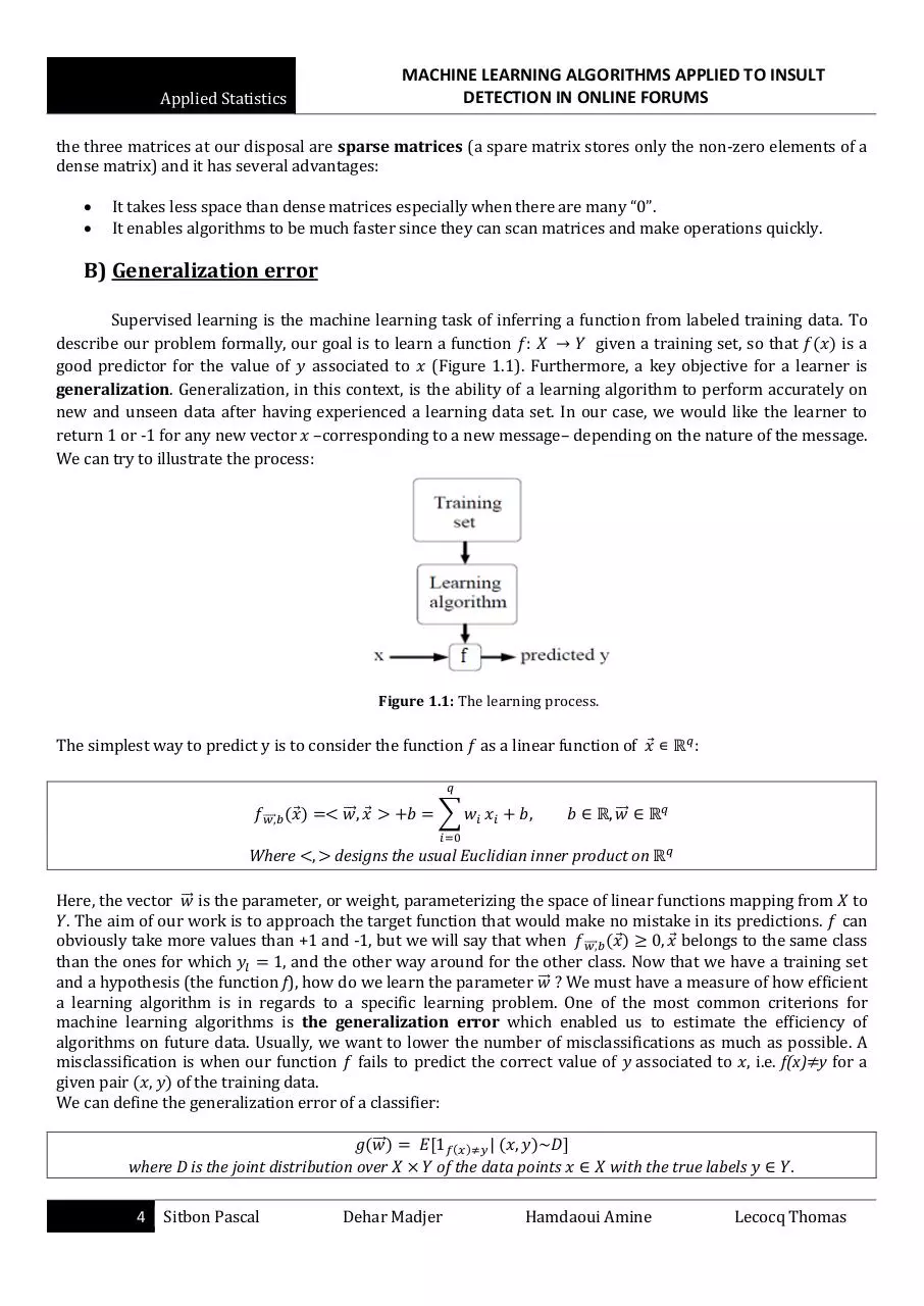
The simplest way to predict y is to consider the function

⃗⃗⃗⃗

( )

Where

⃗⃗

as a linear function of

∑

:

⃗⃗

designs the usual Euclidian inner product on

Here, the vector ⃗⃗ is the parameter, or weight, parameterizing the space of linear functions mapping from to
. The aim of our work is to approach the target function that would make no mistake in its predictions. can
obviously take more values than +1 and -1, but we will say that when ⃗⃗⃗⃗ ( )
belongs to the same class
than the ones for which
, and the other way around for the other class. Now that we have a training set
and a hypothesis (the function f), how do we learn the parameter ⃗⃗ ? We must have a measure of how efficient
a learning algorithm is in regards to a specific learning problem. One of the most common criterions for
machine learning algorithms is the generalization error which enabled us to estimate the efficiency of
algorithms on future data. Usually, we want to lower the number of misclassifications as much as possible. A
misclassification is when our function fails to predict the correct value of associated to , i.e. f(x) y for a
given pair (
) of the training data.
We can define the generalization error of a classifier:
( ⃗⃗ )
where D is the joint distribution over
4

Sitbon Pascal

( )
( )
of the data points

Dehar Madjer

with the true labels

Hamdaoui Amine

.

Lecocq Thomas

Applied Statistics

MACHINE LEARNING ALGORITHMS APPLIED TO INSULT
DETECTION IN ONLINE FORUMS

Finding an analytic expression of is key since it makes it easy to find the vector ⃗⃗ that defines our function .
Indeed it will be the vector that minimizes the generalization error. However, we generally do not know the
{(⃗⃗⃗ )
distribution of points. So we try to minimize a function ĝ on the training set
{
} ⃗⃗⃗
}. The first idea we had was to minimize the
loss on the training dataset but this problem
is quite difficult since the loss function is not convex. In order to use well-known algorithms for optimization,
we need to be a convex function.
Then we chose a usual analytic expression for :
( ⃗⃗ )

∑ (⃗⃗⃗

⃗⃗ )

Where l is a convex loss function that approximates the

loss.

This function is also called the empirical loss. It should be underlined that is only an estimator of the true
generalization error and minimizing does not necessarily imply minimizing the real generalization error.
Sometimes, when learning is performed too long, the algorithm may adjust to very specific random features of
the training data that have no causal relation to the target function. Then the training error decreases and the
validation error increases while the percentage of the dataset used to constitute the training dataset increases
(i.e. the learning algorithm trains more). This phenomenon is called overfitting (Figure 1.2).

Figure 1.2: Misclassification on test and training set depending on the % of data used to constitute the training
data.

The concept of overfitting is important in machine learning. Overfitting happens when the vector ⃗⃗ is too
complex (i.e. when its norm is too larger). Then the vector ⃗⃗ is too specific to a model and the learning
algorithm will give us low results on unseen data. One usual way of avoiding overfitting is regularization.

C) Regularization and Gradient method
Regularization consists in adding an extra term to the error function in order to penalize complex ⃗⃗
vectors. Let’s call r this function, note that it is a function of ⃗⃗ . The function r can take different forms, most of
the time it is the or norm of ⃗⃗ . Even if it can seem arbitrary, it can be shown that it minimizes the influence
of spurious correlations in the training set. Indeed, it limits the complexity of the model since ‖ ⃗⃗ ‖ would be
larger when vector ⃗⃗ is more complex. Our new error function can be defined as follows:
5

Sitbon Pascal

Dehar Madjer

Hamdaoui Amine

Lecocq Thomas

MACHINE LEARNING ALGORITHMS APPLIED TO INSULT
DETECTION IN ONLINE FORUMS

Applied Statistics

( ⃗⃗ )

∑ (⃗⃗⃗

⃗⃗ )

( ⃗⃗ )

Now that we have our optimization problem, we need a method to minimize i.e. to find ⃗⃗
( ⃗⃗ ). A
classical mathematical method to find the minimum of a function is gradient descent. This method is based on
the fact that the gradient
of a function points in the direction of the greatest increase so that
points in
the direction of the greatest decrease. Then a natural iterative algorithm is to update an estimate ⃗⃗ :
∑

(⃗⃗⃗

⃗⃗ )

This update is simultaneously performed for all values of
Here, is the learning rate, it determines how far we move in the direction of the gradient. It is a key
parameter. Indeed, it should not be too small if we do not want the algorithm to be too long and it should not be
too large if we do not want to miss the minimum. This method looks at every example in the entire training set
on every step, and is called the Batch gradient descent. The ellipses shown below are the contours of a
quadratic function (Figure 1.2). Also shown is the trajectory taken by the gradient descent method.

Figure 1.3: The gradient descent trajectory. (Adapted from reference [1])

Note that the gradient descent is deterministic, which means that every time we run for a given training set, we
will get the same optimum in the same number of iterations. However, when our training sample is very large,
this method may take too long because in every iteration we are running through the complete training set.
There is an alternative to the Batch gradient descent that also works very well and avoid running
through the entire training set, consider the following algorithm:
(⃗⃗⃗

⃗⃗ )

Where is an index drawn randomly at each step from {
This update is simultaneously performed for all values of

}

In the gradient descent, we compute the gradient using the entire training set. In this algorithm, we
approximate the gradient by using a single example of the training data set. This technique is called the
stochastic gradient descent method. We run through the training set and every time we find a training example,
we update the parameters according to the gradient of the error with respect to that single training example
only. As we use only a single example each time we are only getting an approximation to the true gradient, then
we do not have any guarantee of moving in the direction of the greatest descent. Nevertheless, there are at least
two reasons why stochastic gradient descent is always useful for large-scale learning problems. First, it is way
quicker than the Batch gradient descent method when is large. On the other hand, it can be shown that the
stochastic gradient descent often gets close to the minimum much faster than the usual gradient descent.
6

Sitbon Pascal

Dehar Madjer

Hamdaoui Amine

Lecocq Thomas

Applied Statistics

MACHINE LEARNING ALGORITHMS APPLIED TO INSULT
DETECTION IN ONLINE FORUMS

Actually, it may never “converge” to the minimum since it uses an approximation of the gradient so the
parameter ⃗⃗ will keep oscillating around the minimum; yet, in practice, the values near the minimum will be
good-enough approximations of the real minimum. For instance, the trajectory shown below is the trajectory
taken by the stochastic gradient descent method (Figure 1.3).

Figure 1.4: The stochastic gradient descent trajectory. (Adapted from reference [1])

In 2008, Leon Bottou (Princeton) and Olivier Bousquet (Google) published a paper called The Tradeoffs of Large
Scale Learning to show concretely how a learning algorithm can be poor at optimization but excellent when it
comes to generalization. They developed a framework that explicitly includes the effect of optimization error in
generalization and then they analyzed the asymptotic behavior of this error when the number of training
examples is large. They did it by looking at the estimation error which is intuitively a measure of how
representative of the implicit distribution the training set is. When they compared the results obtained by the
Batch gradient descent and the results obtained thanks to the stochastic gradient descent, their conclusion was
that the stochastic gradient algorithms benefit from their lower estimation error in large datasets to achieve a
low generalization error quicker than basic gradient descent algorithm. One of the key interrogations of this
paper is the question of how useful approximate solutions are to learning problems: what is the cost in term of
generalization errors if we only approximately solve the optimization problem that models our goal? The
authors answered this question by showing that we do not need to focus on precise solutions –in large-scale
learning–since it is possible to achieve low generalization error without deterministic solutions. This is
something interesting –one can have a look at the original document for more mathematical details- and should
be underlined since it is not common in computer science. Indeed, most of the time, the optimization problem is
the problem of interest while in learning the real quantity of interest is the generalization error. As we saw, the
optimization formulation of the problem is only a compensation for the fact we never know the underlying
distribution of the test data. Actually, this is one of the key contributions of Bottou and Bousquet’s paper.
Even though stochastic gradient descent has been around in the machine learning community for a long time, it
has received a considerable amount of attention in the context of large-scale learning just recently. Indeed, its
iteration complexity is independent of while the Batch gradient descent complexity is linear in . Most of the
algorithms in the methods we study such as SVM and logistic regression use variants of the stochastic gradient
descent. This is something clear when we look at Scikit-Learn algorithms. Scikit-Learn is an open source
machine learning library for the Python programming language that we use for our work.
However, the stochastic gradient descent has a few drawbacks:
 It is sensible to feature scaling which is not an issue for us since our dataset is already normalized.
 The loss function and the regularization function must be convex functions.
 It requires a number of parameters such as the regularization function and the number of iterations.

7

Sitbon Pascal

Dehar Madjer

Hamdaoui Amine

Lecocq Thomas

MACHINE LEARNING ALGORITHMS APPLIED TO INSULT
DETECTION IN ONLINE FORUMS

Applied Statistics

II.

SOME WELL-KNOWN CLASSIFIERS
NB: In II) and III) we will use the same training set and the same test set in order to compare the different
classifiers. In order to do so, we set a random seed in the algorithm used for creating the training and test
datasets. A random seed is a number used to initialize a pseudorandom number generator. We used the
seed “0” throughout this paper. We decided use 60% of the data set for the training set and 40% for the
test set as it is usually done for datasets that contain approximately as many data points as our data set.

This part will present three of most well-known classifiers: Support vector machines, decision trees and logistic
regression. For each classifier we will some key points of the theory necessary to understand the simulations
and how the classifier is obtained.
The two most common indicators that allow oneself to evaluate the efficiency of a classifier on a set are the
misclassification rate and the recall rate. The first one is the number of messages that wrongly predicted in this
set:
Misclassification Rate:
Accuracy =

Misclassification Rate

Here we are tracking insults; the recall rate therefore indicates the percentage of insults captured in this set:
Recall Rate:

A) Support Vector Machines
The principal goal of SVM is to find a “good” separation between the two classes (insulting or clean
messages for us); this separation is then used to make predictions. Indeed, messages from a training data set
are mapped into a specific space (which axes are the variables in our matrix), the algorithm finds a hyperplan
which separate the messages of the two classes in a “good” way. Then if a new message is given, his predicted
class will depend on his position with regard to the hyperplan.

1) Theory
As written in part I, a data set containing points which belong to two classes can be represented by the
following set:
{(

{

)

is a message for
represents the belonging to one of the two classes (
is the number of data points (Number of messages)
is the number of features observed for each message

}

if

}(

)

is an insult, else

)

The easier example to give is a linearly separable set, then we will see how to deal with a data set which points
are not linearly separable, and even not separable (which is more often the case when the data set contains a
reasonable number of points)
8

Sitbon Pascal

Dehar Madjer

Hamdaoui Amine

Lecocq Thomas

MACHINE LEARNING ALGORITHMS APPLIED TO INSULT
DETECTION IN ONLINE FORUMS

Applied Statistics


Linearly separable set

On Figure 2.1 it’s easy to see that the data points can be linearly separated. But, most of the time with a big data
set, it’s impossible to say just by visualizing the data that it can be or not linearly separated, even the data can’t
be visualized in fact.

Figure 2.1: A linearly separable set (D).

Let’s give some definitions necessary to understand and solve the problem analytically:
Notation:

will design the usual Euclidian inner product on

Definition: A linear separator of
is a function
and
. is given by the following formula:

which depends on two parameters that we will note ⃗⃗

( )

⃗⃗⃗⃗

and ||.|| the associated norm.

, ⃗⃗

⃗⃗

This separator, can take more values than +1 and -1, but we will say that, when ⃗⃗⃗⃗ ( )
belongs to the
same class than the ones for which
, same comment for the other class. The line of separation is the
contour line defined by: ⃗⃗⃗⃗ ( )
.
Definition: The margin of an element (

} relatively to a separator , noted

{

)

(

)

, is a real

given by the following formula:

(

Definition: The margin is linked to a separator
)
couples (
:

)

( )

and a set of points , it is the minimum of the margin of each

{

(

Definition: The support vectors are the ones for which:

)

(

(

)

}
)

, i.e. :

(

)

.

Intuitively, the support vectors are the ones which have an impact on the hyperplan boundary (Figure 2.2),
removing or moving support vector will change the equation of the sparating hyperplan.
9

Sitbon Pascal

Dehar Madjer

Hamdaoui Amine

Lecocq Thomas