GP04 (PDF)

driven
harmonic
motion
revised KLA November 2015

GP04

Handle the Driven Harmonic Motion apparatus carefully. It is delicate and if it breaks, recoiling
cords and dropping weights could present a hazard.

1

Introduction
The aim of the experiment is to test the mathematical theory of a damped harmonic oscillator, both
the free oscillation, and the response to a driving force over a wide range of frequencies. The spring
constant, the mass and the damping constant are measured independently, allowing quantitative comparison of theory and experiment. The system to be studied is a mass m suspended on a vertical spring.
The displacement from equilibrium x is measured, and the system can be driven by displacing the suspension point of the spring by a distance y(t) relative to equilibrium. The spring is assumed to obey
Hooke’s Law, acting on the mass with a force F = −k(x − y). In addition there is a magnetic damping
˙ with B a constant and the dot indicating differentiforce on the mass proportional to the velocity −B x,
ation with respect to time. In free oscillations y = 0 and we study x in terms of k, m, B and the initial
conditions. In driven oscillations we study x for the case y = y0 cos(ωt) for a range of frequencies ω.

2

Theory
The equation of motion of a free damped simple harmonic oscillator comes from Newton’s Second Law:
m x¨ = −kx − B x˙

(1)

If the support point of the spring is moved then the restoring force is k(x − y) instead of kx, giving the
equation for forced motion:
m x¨ + B x˙ + kx = ky(t)
(2)
The solution of this consists of the sum of two parts; the particular integral or steady state solution
(with no arbitrary constants) and the complementary function or transient solution, with two arbitrary
constants, determined from the initial conditions.
Let B = mγ, k = mω02 , and y(t) = y0 cos ωt, then the associated complex equation for equation 2 becomes:
z¨ + γz˙ + ω02 z = ω02 y0 eiωt
(3)
The complementary function is the solution to the equation of motion with y = 0, corresponding to
y0 = 0 in equation 3. Substituting z = Aeiωt gives:
− ω 2 + iγω + ω02 = 0
10Nov2015

Copyright © 2015 University of Oxford, except where indicated.

(4)
GP04- 1

driven harmonic motion

So
ω=

iγ
γ2 1
± (ω02 − ) 2
2
4

(5)

z = e− 2 (Ceiωγ t + De−iωγ t )
γt

2

(6)

1

γ
2
where ωγ = ω0 (1 − 4ω
2) .
0

The displacement x is the real part of z and can be expressed as:
x = Ee− 2 cos(ωγ t + θ)
γt

(7)

Note that because of the e− 2 factor this contribution to the displacement x dies away in a characteristic
time γ2 .
γt

For the particular integral, y0 ≠ 0 in equation 3. Substituting z = Aeiωt gives:
A(−ω 2 + iγω + ω02 ) = ω02 y0

(8)

So
A = y0

ω02
(ω02 − ω 2 ) + iγω

= y0

ω02 ((ω02 − ω 2 ) − iγω)
(ω02 − ω 2 )2 + ω 2 γ2

= y0

ω02 e−iφ
1

[(ω02 − ω 2 )2 + ω 2 γ2 ] 2

,

(9)

where φ is the phase lag of the response and is given by:
tan φ =

ωγ
(ω02 − ω 2 )

.

(10)

However, as you know, this equation is ambiguous as to the quadrant φ is in. The correct phase varies
from zero at zero driving frequency to +π at infinite driving frequency. This is correctly given by the
√
principal branch of the equation φ = arccos [(ω02 − ω 2 )/ (ω02 − ω 2 )2 + ω 2 γ2 ]
The amplitude of the response is
∣ A ∣≡ x0 = y0

ω02
1

[(ω02 − ω 2 )2 + ω 2 γ2 ] 2

,

(11)
2

∂∣A∣−2

1

2
which has a maximum when ∂ω = 0, i.e. −4ω(ω02 − ω 2 ) + 2ωγ2 = 0. So ωmax
≡ ωR = (ω02 − γ2 ) 2 , which
is one definition of the resonant frequency. (This differs from ωγ ; however other definitions of ω R give
ω R = ωγ .)

Thus A = x0 e−iφ , and the displacement x is given by
x = x0 cos(ωt − φ)
with x0 given by equation 11 and φ by equation 10. In terms of the Quality Factor Q =
ment x can be written
ω02
x = y0 cos(ωt − φ)
.
1
0 2 2
[(ω02 − ω 2 )2 + ( ωω
)
]
Q

(12)
ω0
γ

the displace(13)

(Strictly speaking Q should be defined as ωγ /γ, but the distinction is usually too small to be significant,
and the above is the form most often quoted.)
GP04-2

Copyright © 2015 University of Oxford, except where indicated.

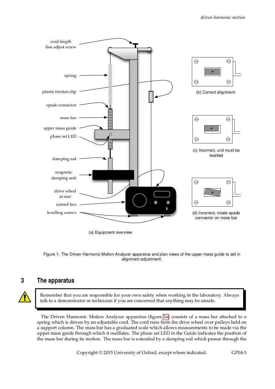
driven harmonic motion

cord length
fine adjust screw

spring

plastic friction clip

(b) Correct alignment

spade connector
mass bar
upper mass guide
phase set LED
(c) Incorrect, unit must be
levelled

damping rod
magnetic
damping unit
drive wheel
at rear
control box
levelling screws

(d) Incorrect, rotate spade
connector on mass bar

(a) Equipment overview

Figure 1: The Driven Harmonic Motion Analyzer apparatus and plan views of the upper mass guide to aid in
alignment adjustment.

3

The apparatus
Remember that you are responsible for your own safety when working in the laboratory. Always
talk to a demonstrator or technician if you are concerned that anything may be unsafe.
The Driven Harmonic Motion Analyzer apparatus (figure 1a) consists of a mass bar attached to a
spring which is driven by an adjustable cord. The cord runs from the drive wheel over pulleys held on
a support column. The mass bar has a graduated scale which allows measurements to be made via the
upper mass guide through which it oscillates. The phase set LED in the Guide indicates the position of
the mass bar during its motion. The mass bar is extended by a damping rod which passes through the
Copyright © 2015 University of Oxford, except where indicated.

GP04-3

driven harmonic motion

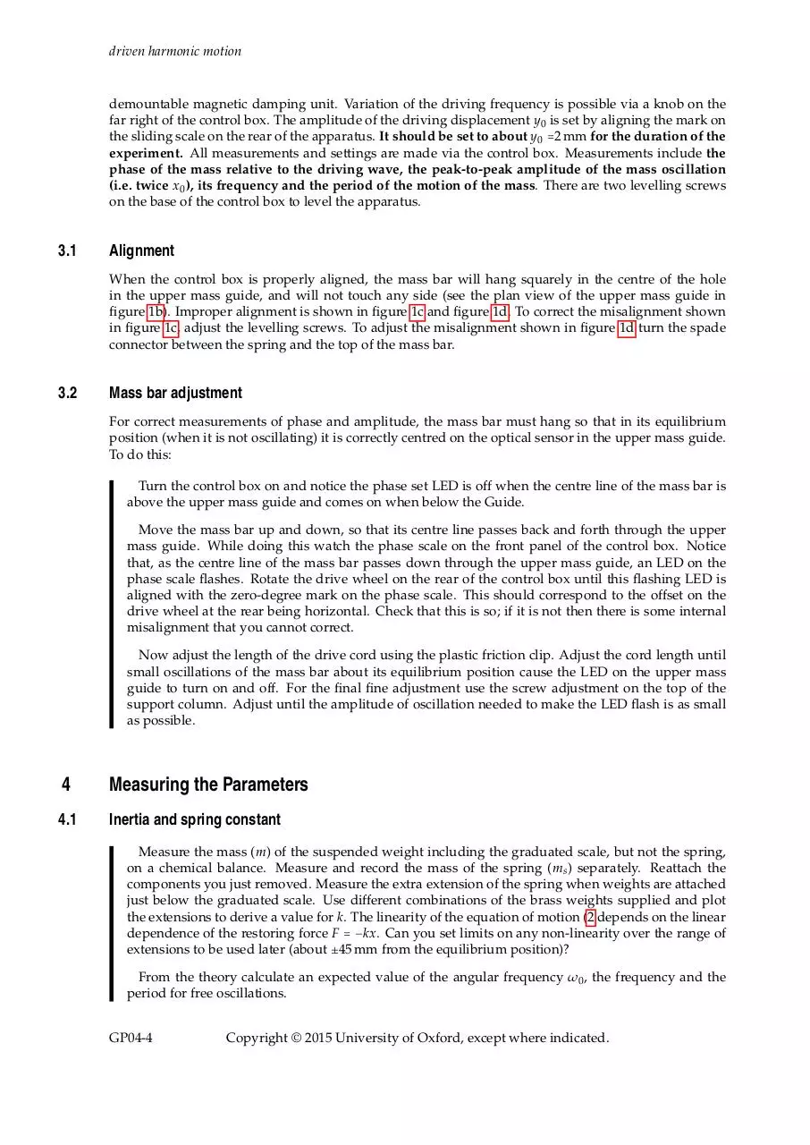
demountable magnetic damping unit. Variation of the driving frequency is possible via a knob on the
far right of the control box. The amplitude of the driving displacement y0 is set by aligning the mark on
the sliding scale on the rear of the apparatus. It should be set to about y0 =2 mm for the duration of the
experiment. All measurements and settings are made via the control box. Measurements include the
phase of the mass relative to the driving wave, the peak-to-peak amplitude of the mass oscillation
(i.e. twice x0 ), its frequency and the period of the motion of the mass. There are two levelling screws
on the base of the control box to level the apparatus.

3.1

Alignment
When the control box is properly aligned, the mass bar will hang squarely in the centre of the hole
in the upper mass guide, and will not touch any side (see the plan view of the upper mass guide in
figure 1b). Improper alignment is shown in figure 1c and figure 1d. To correct the misalignment shown
in figure 1c, adjust the levelling screws. To adjust the misalignment shown in figure 1d turn the spade
connector between the spring and the top of the mass bar.

3.2

Mass bar adjustment
For correct measurements of phase and amplitude, the mass bar must hang so that in its equilibrium
position (when it is not oscillating) it is correctly centred on the optical sensor in the upper mass guide.
To do this:
Turn the control box on and notice the phase set LED is off when the centre line of the mass bar is
above the upper mass guide and comes on when below the Guide.
Move the mass bar up and down, so that its centre line passes back and forth through the upper
mass guide. While doing this watch the phase scale on the front panel of the control box. Notice
that, as the centre line of the mass bar passes down through the upper mass guide, an LED on the
phase scale flashes. Rotate the drive wheel on the rear of the control box until this flashing LED is
aligned with the zero-degree mark on the phase scale. This should correspond to the offset on the
drive wheel at the rear being horizontal. Check that this is so; if it is not then there is some internal
misalignment that you cannot correct.
Now adjust the length of the drive cord using the plastic friction clip. Adjust the cord length until
small oscillations of the mass bar about its equilibrium position cause the LED on the upper mass
guide to turn on and off. For the final fine adjustment use the screw adjustment on the top of the
support column. Adjust until the amplitude of oscillation needed to make the LED flash is as small
as possible.

4

Measuring the Parameters

4.1

Inertia and spring constant
Measure the mass (m) of the suspended weight including the graduated scale, but not the spring,
on a chemical balance. Measure and record the mass of the spring (ms ) separately. Reattach the
components you just removed. Measure the extra extension of the spring when weights are attached
just below the graduated scale. Use different combinations of the brass weights supplied and plot
the extensions to derive a value for k. The linearity of the equation of motion (2 depends on the linear
dependence of the restoring force F = −kx. Can you set limits on any non-linearity over the range of
extensions to be used later (about ±45 mm from the equilibrium position)?
From the theory calculate an expected value of the angular frequency ω0 , the frequency and the
period for free oscillations.
GP04-4

Copyright © 2015 University of Oxford, except where indicated.

driven harmonic motion

· The theory of 2 assumes a massless spring. The correction for the mass of the spring is to
replace m by m + 13 ms . Calculate values and errors for ω0 using both formulae. Is the difference
significant?

4.2

Period of free oscillations without damping
Remove the magnet assembly. Check the alignment of the apparatus (section 3.1 and 3.2) ensuring
that the drive is not- switched on. Switch the function switch to period. Pull the mass bar down by
about 50 mm and release. Record the period indicated in seconds.

· Comment on the accuracy of the period obtained, and compare this result with the predicted
value.
4.3

Period and decay of free oscillations with damping
Secure the magnet assembly in position and adjust the magnets so that the distance between the
poles is about 14 mm and the poles are equidistant from the bar. Repeat the alignment procedure
(section 3.1 and 3.2). Keep the drive switched off. Set the function switch to amplitude. Pull the mass
bar down to start free oscillations. Ignore the first swing, for which the digitisation of amplitude is
spurious. Record the amplitude of the second and subsequent oscillations. (You will need to find a
reliable procedure for recording the data as they are displayed. You can try recording alternate ones
with your partner, or filming the decay with a mobile phone.) Record the readings in a table in your
logbook and repeat several times.
Now you need to get your data into a format ready to analyse on the computer. There are two ways to
do this and you can choose which you prefer.
The first way is to enter your readings directly into RStudio using its spreadsheet functionality.
Firstly open RStudio. If you want to put your data into a folder called mydata then you need to type
mydata=data.frame() (to create a blank ”data frame”, which is like a spreadsheet), and to enter the
data then type mydata=edit(mydata). A spreadsheet-like window should appear in which you can
enter the data. It is best to rename the labels var1 to something more relevant to your experiment.
This data is now ready to process straight away in RStudio, but it is a good idea to save your data as
well using the command write.csv(mydata, file="GP04data.csv") which should put a file called
GP04data.csv into your home directory.
The second way is to enter your readings into a spreadsheet program and save as a Comma Separated Value (.csv) file.
Use the theory of section 2 to show that the peak-to-peak amplitude of the nth successive oscillation
decays as e−nπ/Q . Fit your data to an exponential decay using the RStudio code GP04 expfit.R, which
is located in the GP04 folder in the S: (shared) drive.
This file can be opened by either double clicking straight on it, or running RStudio and then clicking
and choosing the file. Before you do anything else, save your edited version of the the prewritten code with another file name in your home drive.
Open File

If you made a CSV file of your data to read in above, you can use the Import Data command as you
did in DA01 to read in the data. If you made your data file directly in RStudio you can skip this part.
In both cases, make sure the names for your data are consistent with the rest of the code. (Remember
you can access the first column of mydata, called x, by typing mydata$x).
Copyright © 2015 University of Oxford, except where indicated.

GP04-5

driven harmonic motion

From the exponential decay constant derive values (with errors) for Q from each of your data sets
(assume a constant y-error of 1 mm).

· Are the decay data consistent with the exponential function? Are the different values for Q
consistent? How should they be combined to derive a single best value from your measurements?

Use Q to derive values for γ and B with errors. Calculate the damped frequency ωγ . Remeasure it as
in section 4.2 and comment on your results. Is the difference from ω0 significant?

· Discuss your work with a demonstrator.

5

Comparing experiment and theory

5.1

Taking Data for Amplitude and Phase
Check that the drive amplitude is about 2 mm, and recheck the alignment (section 3.1 and 3.2). Turn
the drive on. The behaviour of the oscillator will now be described by a superposition of steady state
and transient solutions. From the existing results, calculate how long the transient solution takes to
decay away to less than 2% of its initial value after switching on. When taking readings in the steady
state, wait at least this long for the motion to stabilise.
Record the phase and amplitude of the oscillation in a table, as a function of frequency (note that the
number displayed is peak-to-peak amplitude or 2x0 ). Start at a frequency of 0.7 Hz increasing in steps of
0.2 Hz up to at least 3.0 Hz. In the region of the resonance around 1.8 Hz it will be necessary to take finer
steps of 0.1 or even 0.05 Hz to record the detail. Record phase data with lagging phases as positive to
be consistent with the theory of section 2. If you observe small leading phases at low frequency, record
these as negative, and if you observe large leading phases at high frequency, such as −150°, record these
as positive phases by adding 360° to get 210°.
Enter your frequency, amplitude and phase data into the RStudio spreadsheet, or alternatively save it
in CSV format.

5.2

Fitting the Amplitude Data
The amplitude is fitted with a peak function, given by
y(x) =

k
[(xc2 − x2 )2 + x2 w2 ]1/2

(14)

which you can compare with equation 11.
Here, k is a constant and interpretation of the parameters xc and w depends on the form in which
you enter your data. If you enter angular frequencies ω for x, then xc will be ω0 and w will be γ.
Alternatively, if you enter frequencies f = ω/(2π), then xc and w will also be scaled by 2π.
The RStudio code GP04 Amp PhaseFit.R has been written to determine values for ω0 , γ and the drive
amplitude y0 .
Load it up in RStudio from the GP04 folder in the S: shared drive, using the same approach as in
section 4.3. Don’t forget to save the script with a different name in your home area before going any
further.
GP04-6

Copyright © 2015 University of Oxford, except where indicated.

driven harmonic motion

As above, use the Import Data command or enter the data in the RStudio spreadsheet - remember
you are likely to need to edit the variable names so that they are consistent. You may need to play
with the header and skip commands to read in the right data and make sure your header row is in
the right place.
Run Part 1 of the code to fit the amplitude data and plot your data as points with the fit overlain as
a line. Look at the standard error in the fit parameters with summary(fit), where fit is the name of
your fit. Also examine the residuals; they can be visualised using plot(residuals(fit)).

· Comment on the accuracy of the fit.

5.3

Fitting the Phase Data
The phase data are fitted with the following function:
y(x) = arccos[(xc2 − x2 )/s] + [esys s/xc2 ] + y0

(15)

where s = [(xc2 − x2 )2 + x2 w2 ]1/2 . Compare equation 15 with equation 10. The two parameters xc and w
correspond to the same parameters in the amplitude fit, and Q is calculated from them in the same way.
The two parameters esys and y0 should initially be fixed to zero, but can be used to fit systematic errors
in the phase measurement. Code has been written for you in Part 2 of GP04 Amp PhaseFit.R to do this.
We have written two versions of equation 15, one with the error term included and one without. Check
you understand which is which.
Fit the phase data, using the version without the error terms, to implement the theoretical prediction.
The data must use the sign convention discussed above. Plot the data showing the fit.

· Comment on the accuracy of the fit by looking at the standard errors and residuals. Are the
deviations from the fit random, and consistent with the precision of the phase measurements?

It is likely that the phase data will fit significantly worse than the amplitude data, because of systematic
errors in the phase measurement. The phase measurement relies on two separate alignments:
1. The null-point of the drive must occur when the rotor inside the control box which carries the
phase display LED is passing zero. Any error here leads to a constant phase error which is fitted
with y0 , which is the misalignment in degrees.
2. The triggering of the LED should occur at the zero-point of the oscillation. Any error here leads to
an amplitude-dependent error which is fitted with esys , which is the offset of the trigger point as a
multiple of the drive amplitude ydrive .
Re-fit the phase data using the equation that includes the error terms. Determine values of ω0 and
γ from the phase fit. Draw the new phase fit as a line of a different colour on your plot. Draw up a
table of values to compare ω0 , γ as derived from the direct measurement of parameters in sections 4.1
and 4.3, from the amplitude data in section 5.2, and from the phase data in this section.
Compare the different values and their errors directly in RStudio for each parameter. Do this by
plotting the various values (used as the Y axis) and their errors, against a list of integers 1, 2, 3 etc. (used
as the X axis). These can be fitted with a straight line with zero slope, using the command sequence
lm(Y∼offset(0*X)). The fit diagnostics will then disclose whether the different values are consistent.
Copyright © 2015 University of Oxford, except where indicated.

GP04-7

driven harmonic motion

· Do your data give support for the correction for the spring mass? Do they give support for the
coefficient 13 ?

· Now hand-write a brief summary of the experiment in your logbook. State the aims of the experiment, the method used, quantitative results, and whether you consider that the experiment
has verified the theory. Discuss the reasons for any discrepancies between theory and experiment. This should take no more than about half a page. Show this to a demonstrator as part of
your assessment.

GP04-8

Copyright © 2015 University of Oxford, except where indicated.