emloyment analysis (PDF)
File information
Author: Aleksandar
This PDF 1.5 document has been generated by Acrobat PDFMaker 15 for Word / Adobe PDF Library 15.0, and has been sent on pdf-archive.com on 29/05/2016 at 15:31, from IP address 71.227.x.x.
The current document download page has been viewed 2538 times.
File size: 173.31 KB (9 pages).
Privacy: public file


File preview
All data used in this analysis comes from the U.S. Bureau of Labor Statistics (“BLS”) and U.S. Bureau of
Economic Analysis (“BEA”).
1. Narrowing the scope down to occupations that don’t require higher level of education
In defining what “don’t require” means, let’s start looking at some data first. BLS provides data on
educational levels by occupation ranging from CEOs and lawyers to farmers and parking lot attendants.
BLS shows the distribution of educational levels by occupation. The example distribution for CEOs can be
seen in the table below. Evidently, 69% of CEOs have received a Bachelor’s degree or higher.
Educational level
Less than high school diploma
High school diploma or equivalent
Some college, no degree
Associate's degree
Bachelor's degree
Master's degree
Doctoral or professional degree
Percent of CEOs
1.5%
9.2%
15.2%
5.3%
40.3%
21.3%
7.2%
To unpack this data, let’s combine Associate’s degree or lower (“Lower education”) and Bachelor’s
degree or higher (“Higher education”), as shown in the table below.
Educational level
Lower education
Higher education
Percent of CEOs
31.2%
68.8%
Further, let’s assume a certain length of education per level to get the average length of education per
occupation.
Educational level
Less than high school diploma
High school diploma or equivalent
Some college, no degree
Associate's degree
Bachelor's degree
Master's degree
Doctoral or professional degree
Assumed years of education
8
12
13
14
16
18
20
So our two metrics for CEO then are 68.8% higher education, and 15.7 years of education on average.
The below chart plots these two metrics for all occupations in the data set.
Educational levels by occupation
20
Avg. years of education
18
16
14
12
10
8
0%
20%
40%
60%
Proportion higher education
80%
100%
Now armed with some data, we can start creating our own definition of what don’t require higher
education means. The chart shows the distribution two types of curvatures – a high slope in the
beginning and end of the curve, indicating pockets of low vs. high levels of required education. The
middle section exhibits a flatter slope. The beginning of the flattening out part of the curve starts around
25% of proportion of higher education. Let’s further pick the semi-arbitrary number of 13 years of
education, at the educational attainment level “some college, no degree.”
So our working definition is don’t require higher education means the educational profile of the
occupation has both below 13 years of education on average and below 25% of higher educated
workers. While this may sound like a tough criteria, it only eliminates 61% of occupations, leaving a total
of 39% left. That’s almost half of all kinds of jobs that are up for grabs.
2. Identifying occupations with attractive employment characteristics
a. Income relative to education
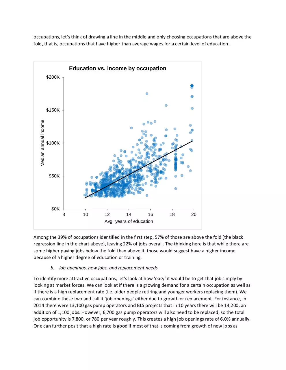
It makes sense that the more you study, the higher degree of specialization you attain, and as such
command a higher wage. Plotting the median income against average length of education shows this
positive trend. There is a certain ‘return on your investment’ with respect to education. That being said,
for the same amount of education, some occupations pay more and some pay less. To shortlist
occupations, let’s think of drawing a line in the middle and only choosing occupations that are above the
fold, that is, occupations that have higher than average wages for a certain level of education.
Education vs. income by occupation
$200K
Median annual income
$150K
$100K
$50K
$0K
8
10
12
14
16
Avg. years of education
18
20
Among the 39% of occupations identified in the first step, 57% of those are above the fold (the black
regression line in the chart above), leaving 22% of jobs overall. The thinking here is that while there are
some higher paying jobs below the fold than above it, those would suggest have a higher income
because of a higher degree of education or training.
b. Job openings, new jobs, and replacement needs
To identify more attractive occupations, let’s look at how ‘easy’ it would be to get that job simply by
looking at market forces. We can look at if there is a growing demand for a certain occupation as well as
if there is a high replacement rate (i.e. older people retiring and younger workers replacing them). We
can combine these two and call it ‘job openings’ either due to growth or replacement. For instance, in
2014 there were 13,100 gas pump operators and BLS projects that in 10 years there will be 14,200, an
addition of 1,100 jobs. However, 6,700 gas pump operators will also need to be replaced, so the total
job opportunity is 7,800, or 780 per year roughly. This creates a high job openings rate of 6.0% annually.
One can further posit that a high rate is good if most of that is coming from growth of new jobs as
opposed to a replacement of older workers. So let’s plot the job market growth rate against the job
openings rate.
Job openings vs. growth by occupation
7%
6%
Job openings rate
5%
4%
3%
2%
1%
0%
-30%
-20%
-10%
0%
10%
20%
30%
40%
Job market growth
We can narrow occupations down to the ones that are at least not shrinking. While the average job
opening rate is 2.8%, we can be a bit more inclusive and set our filter to include occupations that have a
job openings rate of 2% or higher. Adding these filters, excludes 41% of the jobs remaining from the last
step while keeping 59%, or 13% overall.
c. Pay
After all, we are looking at jobs that pay well. So let’s plot annual median wages by percentile.
Income distribution by occupation
$100K
Median annual income
$80K
$60K
$40K
$20K
$0K
0%
20%
40%
60%
80%
100%
Percentile
For our filtering purposes. Let’s cut out half of these, sticking to the remaining jobs that are at the top
half of the income distribution, leaving 7% of occupations overall. These remaining occupations have a
median annual income greater than $41,260.
d. Manual review
A manual review of the remaining occupations revealed that 23% of the remaining jobs were jobs likely
requiring a promotion (e.g. supervisor of mechanics) or more specialized knowledge or training (e.g. ship
engineer). This leaves overall 5% of jobs.
e. Downside risk
A final filter is comparing the median wage with the 10th percentile wage, to assess downside potential.
For example, median income for an electrician was $51,880 meanwhile the 10th percentile only received
$36,420, 30% less. In addition, we can look at how the electrician wages looked like 2 years ago and see
if there was a decline or increase in wages. For the electricians, median wages used to be $49,840 2
years ago, representing a 4% increase.
Downside risk vs. income growth by occupation
$50K
10th percentile annual income
$40K
$30K
$20K
$10K
$0K
-20%
-10%
0%
10%
20%
Median annual income increase/decrease
Let’s further filter down to only include occupations where median income grew and the 10th percentile
income is at least $25K, still leaving 5% of overall occupations.
Remaining is a list of 37 occupations, all covered by 4 of BLS’ major occupational groups, “Construction
and Extraction”, “Installation, Maintenance, and Repair”, “Production”, and “Transportation and
Material Moving”, under major occupation codes 47, 49, 51, and 53. All at a glance physical jobs.
Job
market
growth
Job
market
size
Job
openings
rate
Median
annual
income
Occupation
Code
Elevator installers and repairers
47-4021
13%
21K
3%
$80,870
Electrical power-line installers and repairers
49-9051
11%
119K
5%
$66,450
Petroleum pump system operators
51-8093
2%
42K
4%
$65,190
Boilermakers
47-2011
9%
17K
2%
$60,120
Rail transportation workers, all other
53-4099
3%
3.8K
4%
$59,840
Gas compressor and gas pumping station operators
53-7071
4%
5.1K
5%
$58,350
Rail car repairers
49-3043
2%
22K
3%
$55,570
Rotary drill operators, oil and gas
47-5012
13%
28K
5%
$54,310
Control and valve installers and repairers
49-9012
0%
42K
4%
$54,100
Rail-track laying and equipment operators
47-4061
9%
16K
3%
$52,830
Electricians
47-2111
14%
629K
3%
$51,880
Crane and tower operators
53-7021
8%
46K
4%
$51,650
Millwrights
49-9044
15%
41K
4%
$51,390
Plumbers, pipefitters, and steamfitters
47-2152
12%
425K
2%
$50,620
Structural iron and steel workers
47-2221
5%
61K
2%
$50,490
Commercial divers
49-9092
36%
4.4K
5%
$50,470
Industrial machinery mechanics
49-9041
18%
332K
4%
$49,690
Pile-driver operators
47-2072
16%
3.7K
3%
$49,430
Mobile heavy equipment mechanics
49-3042
5%
125K
3%
$48,770
Reinforcing iron and rebar workers
47-2171
24%
19K
4%
$48,010
Brickmasons and blockmasons
47-2021
19%
78K
3%
$47,950
Derrick operators, oil and gas
47-5011
13%
22K
5%
$47,910
Refractory materials repairers
49-9045
0%
1.8K
3%
$47,060
Wellhead pumpers
53-7073
14%
14K
6%
$46,990
Sheet metal workers
47-2211
7%
141K
3%
$45,750
Heating, AC, and refrigeration mechanics and installers
49-9021
14%
292K
3%
$45,110
Service unit operators, oil, gas, and mining
47-5013
7%
65K
4%
$45,000
Water and wastewater treatment plant operators
51-8031
6%
117K
3%
$44,790
Construction equipment operators
47-2073
10%
363K
3%
$44,600
Extraction workers, all other
47-5099
11%
5.7K
2%
$44,370
Earth drillers, except oil and gas
47-5021
14%
20K
4%
$44,240
Traffic technicians
53-6041
6%
6.8K
6%
$43,930
Insulation workers, mechanical
47-2132
19%
30K
5%
$43,610
Security and fire alarm systems installers
49-2098
13%
64K
4%
$43,420
Maintenance workers, machinery
49-9043
8%
91K
2%
$43,260
Riggers
49-9096
9%
21K
3%
$43,220
Hoist and winch operators
53-7041
0%
2.9K
3%
$42,220
3. Finding the most attractive locations for the jobs
The final step is to take the national level data and apply it to a localized context. Differences in pay, cost
of living (purchasing power), job market saturation, and state income taxes may shed some light on
what jobs to look at and where.
So for this step we will convert gross income to net income at a state level, and normalize the net pay
based on local purchasing power.
The top 10 cities based on average net purchasing power in the collection of the 37 jobs above shown in
the table below. Many of them and other top cities in Illinois.
City
Gross
pay
Net pay
Purchasing
power
Springfield, IL
$64K
$51K
$56K
Kennewick-Pasco-Richland, WA
$64K
$54K
$56K
Danville, IL
$53K
$43K
$55K
Fairbanks, AK
$68K
$57K
$53K
Rockford, IL
$60K
$49K
$53K
Peoria, IL
$58K
$47K
$52K
Anchorage, AK
$68K
$57K
$51K
Michigan City-La Porte, IN
$53K
$44K
$52K
Longview, WA
$57K
$49K
$52K
Champaign-Urbana, IL
$59K
$48K
$51K
The top 3 states are Alaska, Illinois, and Washington. Within these 3 top states, the top jobs by net
purchasing power are shown in the table below.
Job
Gross
pay
Net pay
Purchasing
power
Elevator Installers and Repairers
$83K
$65K
$66K
Electrical Power-Line Installers and Repairers
$80K
$65K
$65K
Hoist and Winch Operators
$87K
$68K
$64K
Service Unit Operators, Oil, Gas, and Mining
$84K
$69K
$62K
Rotary Drill Operators, Oil and Gas
$79K
$65K
$58K
Derrick Operators, Oil and Gas
$78K
$64K
$58K
Plumbers, Pipefitters, and Steamfitters
$65K
$54K
$55K
Insulation Workers, Mechanical
$68K
$56K
$54K
Reinforcing Iron and Rebar Workers
$71K
$58K
$54K
Millwrights
$64K
$53K
$54K
Structural Iron and Steel Workers
$66K
$54K
$54K
Electricians
$63K
$52K
$53K
Brickmasons and Blockmasons
$62K
$50K
$52K
Pile-Driver Operators
$68K
$57K
$52K
Construction Equipment Operators
$61K
$50K
$52K
Crane and Tower Operators
$62K
$51K
$51K
Water and Wastewater Treatment Plant Operators
$60K
$50K
$50K
Rail Transportation Workers, All Other
$65K
$52K
$49K
Control and Valve Installers and Repairers
$62K
$52K
$48K
Petroleum Pump System Operators
$61K
$51K
$47K
Sheet Metal Workers
$55K
$46K
$47K
Boilermakers
$58K
$48K
$47K
Industrial Machinery Mechanics
$54K
$45K
$47K
Earth Drillers, Except Oil and Gas
$58K
$48K
$46K
Heating, AC, and Refrigeration Mechanics and Installers
$53K
$45K
$46K
Mobile Heavy Equipment Mechanics
$53K
$45K
$45K
Security and Fire Alarm Systems Installers
$54K
$45K
$44K
Rail-Track Laying and Maintenance Equipment Operators
$57K
$47K
$44K
Traffic Technicians
$55K
$47K
$44K
Maintenance Workers, Machinery
$48K
$41K
$43K
Rail Car Repairers
$53K
$45K
$42K
Riggers
$51K
$43K
$40K
Refractory Materials Repairers
$47K
$39K
$37K
Finally, if you are on a golden goose chase hunt, the top 10 job-city pairs by purchasing power are shown
in the table below. Location quotient refers to how many such workers are in a given location relative to
that occupation nationally. A number above 1 means a higher concentration of such workers in a city,
and below 1, a lower concentration.
Job
City
State
Gross
pay
Net
pay
Purchasing
power
Location
Electrical Power-Line Installers/Repairers
Kennewick, WA
WA
$88K
$72K
$74K
1.3
Electrical Power-Line Installers/Repairers
Spokane, WA
WA
Electrical Power-Line Installers/Repairers
Wenatchee, WA
WA
$85K
$70K
$72K
0.7
$85K
$70K
$72K
3.5
Millwrights
Kennewick, WA
WA
$84K
$69K
$71K
1.6
Plumbers, Pipefitters, and Steamfitters
Yakima, WA
WA
$82K
$67K
$71K
0.3
Elevator Installers and Repairers
Peoria, IL
IL
$81K
$63K
$69K
2.4
Electrical Power-Line Installers/Repairers
Bellingham, WA
WA
$83K
$68K
$68K
1.3
Plumbers, Pipefitters, and Steamfitters
Rockford, IL
IL
$79K
$62K
$67K
0.6
Electrical Power-Line Installers/Repairers
Springfield, IL
IL
$79K
$62K
$67K
0.8
Electricians
Rockford, IL
IL
$76K
$60K
$65K
1.1
Download emloyment analysis
emloyment analysis.pdf (PDF, 173.31 KB)
Download PDF
Share this file on social networks
Link to this page
Permanent link
Use the permanent link to the download page to share your document on Facebook, Twitter, LinkedIn, or directly with a contact by e-Mail, Messenger, Whatsapp, Line..
Short link
Use the short link to share your document on Twitter or by text message (SMS)
HTML Code
Copy the following HTML code to share your document on a Website or Blog
QR Code to this page

This file has been shared publicly by a user of PDF Archive.
Document ID: 0000378021.