GDMathsGuide (PDF)

Introduction to Mathematics for Game Development.
James Cowley
(Dated: June 6, 2016)

2
I.

INTRODUCTION

This article is intended as an introduction to all the basic mathematical concepts you will need
to understand for game development. It will make the assumption that you are someone who
maybe was never particularly good at maths, or who took maths classes so long ago that you can
barely remember them. Basically, I will not assume much prior knowledge of mathematics.
This guide obviously has it’s limitations; I will not be going into massive depth on any of these
subjects, or treating them with a high degree of rigour. So if you want to get some more details on
any of the topics introduced here, I’ll be providing a reference list at the end.
I’ll wrap up this section with a little bit about myself. I am currently studying physics at
university, in my third year, so maths is like a second language to me (I’m not very good at learning
actual languages, though, unfortunately). I want to go into full-time game development once I
graduate, so I’ve been programming in my spare time, and there are a lot of cases where I have
come across other devs saying “I wish I understood matrices” or “what the hell is a quaternion?”.
So I decided to make this in the hopes that it would help someone out at some point.
Now, on to the meat of the article.

II.

TRIGONOMETRY

I’m sure many of you have traumatic memories of high school trigonometry lessons. That is
fair enough, but trig lies at the heart of a large amount of game development, and maths as a whole.
So you are going to have to take this bull by the horns at some point. I will try to cover it in as
nice a way as possible, though.
Firstly: what is trigonometry? Well, it ultimately stems from the study of geometry, specifically
triangles. The overall idea is to relate angles to distances and vice versa. There are many different
trigonometric quantities, but there are six that you need to know about: sin, cos, tan, arcsin,
arccos, and arctan. They may sound very intimidating, but in reality they are pretty simple, if you
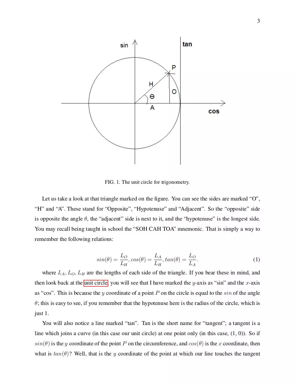
have a diagram to help, that is. If you turn your attention to Figure 1, you will see a construction
called the “unit circle”. The word “unit” is one that crops up all the time in maths; it basically
means “length = 1”. So the unit circle is a circle with a radius of one. Specifically “THE” unit
circle is the circle with radius one, and centred at the origin of whatever coordinate system you are
dealing with.

3

FIG. 1. The unit circle for trigonometry.

Let us take a look at that triangle marked on the figure. You can see the sides are marked “O”,
“H” and “A”. These stand for “Opposite”, “Hypotenuse” and “Adjacent”. So the “opposite” side
is opposite the angle θ, the “adjacent” side is next to it, and the “hypotenuse” is the longest side.
You may recall being taught in school the “SOH CAH TOA” mnemonic. That is simply a way to
remember the following relations:

sin(θ) =

LO
LA
LO
, cos(θ) =
, tan(θ) =
.
LH
LH
LA

(1)

where LA , LO , LH are the lengths of each side of the triangle. If you bear these in mind, and
then look back at the unit circle, you will see that I have marked the y-axis as “sin” and the x-axis
as “cos”. This is because the y coordinate of a point P on the circle is equal to the sin of the angle
θ; this is easy to see, if you remember that the hypotenuse here is the radius of the circle, which is
just 1.
You will also notice a line marked “tan”. Tan is the short name for “tangent”; a tangent is a
line which joins a curve (in this case our unit circle) at one point only (in this case, (1, 0)). So if
sin(θ) is the y coordinate of the point P on the circumference, and cos(θ) is the x coordinate, then
what is tan(θ)? Well, that is the y coordinate of the point at which our line touches the tangent

4
(note we’ll have to continue the line past the unit circle’s edge). Now the unit circle is not great
for finding the exact values of trig functions (except in special cases, such as θ = 90 degrees), but
can come in handy for estimation, and can also give you an intuitive understanding of why some
things occur in trigonometry. For example, if you have a quick look, you will note that if we let
θ = 90 degrees, then sin(θ) = 1,cos(θ) = 0, but you will also notice that no matter how far we
continue our line out, it will never touch the tangent line. so tan(θ) = ∞.
So, let us have an example: say you have an angle of 30 degrees and an adjacent side of length
3 metres. What is the length of the hypotenuse? First, which of the three trig relations involves the
hypotenuse and the adjacent? That would be cos. So the relation for cos is

cos(θ) =

LA
LH

(2)

and we want to get LH . So we multiply both sides by LH :

LH cos(θ) = LA ,

(3)

then divide both sides by cos(θ), to get LH on its own:

LH =

LA
cos(θ)

(4)

and there we have it. We have the unknown (LH ) in terms of known quantities. Plop these into
a calculator and we obtain 3.46 m (to 3 significant figures).
This is all well and good; but if you recall the start of this section, I mentioned six trig quantities.
Where do the “arc”s come in? Well, you may have noticed we have only dealt with finding a length,
given a length and an angle. What if we want to find an angle, given two lengths? This is where
the arc quantities come into play. Arcsin is the “inverse” of the ‘sin function, and similarly for the
other arcs. What does this mean, though? It means that arcsin “undoes” the action of sin. This
will be better illustrated with an example. Say we want to find the angle between the hypotenuse
and the adjacent sides of a triangle. So we want arccos (remember SOH CAH TOA). Let us work
through this step by step:

cos(θ) =

LA
.
LH

(5)

5
We want just θ, so we want to undo the cos. So we apply arccos:
LA
).
LH
Remember that arccos removes the cos, so we just get θ on the left-hand side:
arccos(cos(θ)) = arccos(

(6)

LA
).
(7)
LH
And then, again, the right-hand side is something you can do on a calculator (or in code, e.g.
θ = arccos(

the acos function in C/C++).
Now, any discussion of angles is incomplete without discussing “radians”. The radian is a unit
of angle, just like degrees, except far more useful in mathematics, physics, programming, and
everything really. The basic low-down is that there are 2π radians in a circle, just as there are 360
degrees in a circle. So to convert from degrees to radians, you divide by 180, then multiply by
π. Radians are handy because a lot of mathematical results are neatest, or only work, in radians.
So radians are good to know. Also, some maths functions, e.g. in C and C++, only take radians
as arguments, so you can get all the wrong results if you try using degrees. My advice is to use
radians always, unless you have a specific reason not to.
And that is pretty much it for trigonometry. What do I think you should put emphasis on
learning? The unit circle, SOH CAH TOA, and radians. Learn those and you’re set. Note that
trigonometry goes a whole lot deeper than this, with the hyperbolic functions sinh, cosh, tanh
and so on, but you are very unlikely to need them in game development.

III.

CALCULUS

Calculus is a key part of game programming, especially in physics programming. I am going
to limit this to differential calculus, and you can research integral calculus on your own if you
wish/need to.
Differential calculus is the study of rates. If you are familiar with gradients in geometry, then
finding the gradient of a line is simple differential calculus. You find the change in y, divide it
by the change in x, and that is your gradient. But what if you have a curve? No straight lines
there. This is where you use differentiation. With a curve, we approximate it by assuming that the
curve is made up of an infinite number of infinitesimally small straight lines. Then we say that
the gradient of the curve at a given point is the gradient of the straight line at that point. But how

6
do we work this out practically? Well, say we have a curve described by the equation (this is a
parabola, if you are interested; parabolae come into play with projectiles such as balls or bullets):

y = ax2 ,

(8)

where a is some constant. To differentiate this, we take the power of x (2 in this case) down,
and multiply it with the a, then take one away from the power. That is,
dy
= 2ax1 = 2ax.
dx

(9)

d
(axn ) = naxn−1 .
dx

(10)

In general:

where

d
dx

is the “derivative with respect to x”. It’s as simple as that. From this, you can also

see how to reverse a differentiation, which is called “integration”. I’ll leave that as an exercise for
the reader.
That is pretty much all you need to know about calculus to be starting off with. There is a lot
more you can look into, and what you need to know will be dependent on what sort of things you
want to do. I urge you to look into integral calculus at least.

IV.

IMAGINARY NUMBERS

Imaginary numbers may sound very abstract, but they have many real-world uses, and understanding them is crucial to understanding quaternions (which we’ll be dealing with later), so I shall
give a quick introduction here.
The “imaginary unit”, i, is defined as

i=

√
−1.

(11)

A “complex number” is a number which has an imaginary part and a real part. An imaginary
number is usually denoted by z. So

z = x + iy,

(12)

7
with x being the real component and y the imaginary component. To picture the complex
numbers, you can imagine the usual “real” number line, going from −∞ to ∞. Then, we add a
second line at right-angles to that, to give us the “complex plane”, where the y-axis is the imaginary
axis. In this plane, we represent the complex number z by a point with coordinates (x, y).
If you go back to the unit circle, you can see that we can represent a point in 2D space as a
combination of a sin and a cos term. This can be readily applied to complex numbers, to give us
another representation:

z = |z|(cos(θ) + isin(θ)),

(13)

where |z| is the “magnitude” of z, i.e. the “length” of z, with

|z| =

p
x2 + y 2 .

(14)

The sin, cos representation is called “Euler’s formula”, and provides a very nice geometric
interpretation of complex numbers. The final representation you will want to know is the complex
exponential notation. I assume you are somewhat aware of the number e? If you are not, then it
suffices to say that e has the remarkable quality of being its own derivative:
d x
(e ) = ex .
dx

(15)

In the realm of complex numbers, e has another use:
z = x + iy = |z|eiθ .

(16)

This has an obvious advantage when dealing with differentiation, as differentiating an exponential is pretty easy.
This is pretty much all you will need to know for game development, usually. However, if you
are interested, do check out the internet for some really interesting information.

V.

VECTORS

Now we get to the nitty-gritty of what game dev deals with.
Vectors are a type of mathematical object which have a size, or “magnitude”, and a direction.
Compare that to normal numbers, which are called “scalars”. Those just have a size, and no

8
direction. The difference is best seen in an example: temperature is a scalar; it makes no sense to
say “it is 15 degrees Celsius in the westerly direction”. An example of a vector is displacement,
basically the combination of the distance to something, and the direction to it (e.g. “To get to
that hill, walk 3 kilometres North-West”).
Vectors are represented mathematically in terms of components:

~u = (x, y, z) = x~i + y~j + z~k

(17)

where x, y and z are the components of the vector ~u. ~i, ~j and ~k are the so-called “unit vectors”
(there’s the word “unit” again). These are basically vectors with magnitude 1, pointing in the x,
yand z directions respectively. These are strictly necessary because the (x, y, z) representation is
ambiguous; the x could mean x metres to the left, x metres to the slightly-left-and-behind-you, or
something else entirely. The unit vectors tell you specifically which direction each component is
going in.

A.

Basic Vector Arithmetic

Adding and subtracting vectors is easy; you just go “component-wise”, i.e. adding the x components, adding the ys and so on. You can also multiply and divide vectors by scalars; again we
do this component-wise, so 2~u = (2x, 2y, 2z). However, multiplying two vectors together is more
complicated, as there are two ways in which we can do so: the dot (or “scalar”) product and the
cross (“vector”) product.

B.

Dot Product

Also known as the scalar product, the result of this is a scalar. It basically tells us “how much”
of vector ~u is pointing in the direction of ~v . You can think of this as “projecting” ~u onto ~v . How do
we calculate this? All we do is multiply the x components, the y components and z components,
then add the results together. Simple.
But where do we actually use this in game development? Well, we use it all over the goddamn
place, but two simple example are: you can use it to easily tell if two vectors are perpendicular
(“orthogonal”) to each other; if they are, their dot product will be zero (which is easy to see if you

9
consider the projection of one onto the other). Another simple way the dot product can be used is
in calculating the magnitude of a vector. The magnitude of a three-dimensional vector is given by

|~v | =

p

x2 + y 2 + z 2 .

(18)

Now, you could calculate that manually, but the better way to do it is to take the dot product
of the vector with itself, and square-root that. This is better for two main reasons: firstly, it better
represents the actual mathematical basis. The magnitude of a vector is strictly defined as
|~v |2 = ~v · ~v .

(19)

So using this method just better shows the underlying maths. The other main advantage is that
it gives self-consistency. Ideally, when you are implementing maths in a program, you want it to
be self-consistent. For example (a simple one), you might want to define comparison operators !=
and ==. Now, you could implement them completely separately, but the better way is to define
one in terms of the other. This means that if you do something wrong in programming the first,
you will at least get consistent results in the second; != will still return the opposite of ==, even if
== returns the wrong result.

C.

Cross Product

This is more complicated. This method is also referred to as the “vector product”, because it
returns (shock!) a vector. If the dot product may be thought of as the projection of one vector
onto another, we can picture the cross product as being how much of the first vector is pointing
perpendicular to the other. It returns a vector at right-angles to both the input vectors; this is very
useful throughout physics and game dev. But before we get to uses, let’s see how to calculate it.
There are two ways I use to remember how to do this: the first is more simple, while the second
is more mathematically “rigorous”, as it were. The first method is to imagine a circular route with
“x” at the twelve ‘o’ clock position, “y” at four and “z” at eight. Then imagine arrows going from
x –¿ y –¿ z –¿ x. In order to find the x component of the result, you multiply along the arrows to
get to the x (so you go y times z) and then subtract back along the arrows (subtract z of the first
vector times y of the second vector) and so on. This gets you
~v × ~u = (vy uz − vz uy )~i + (vz ux − vx uz )~j + (vx uy − vy ux )~k.

(20)