report (PDF)

Geostatistical Analysis and Mapping of Ozone in
California, August 2015
Bryan Cole
April 2016

1

Contents
1 ABSTRACT

3

2 INTRODUCTION

4

2.1

Motivation and Problem Statement . . . . . . . . . . . . . . . . .

4

2.2

Research Questions . . . . . . . . . . . . . . . . . . . . . . . . . .

4

3 STUDY AREA AND DATA DESCRIPTION

5

3.1

Study Area . . . . . . . . . . . . . . . . . . . . . . . . . . . . . .

5

3.2

Data Description . . . . . . . . . . . . . . . . . . . . . . . . . . .

6

3.2.1

Ozone monitoring . . . . . . . . . . . . . . . . . . . . . .

6

3.2.2

Elevation data . . . . . . . . . . . . . . . . . . . . . . . .

6

3.2.3

Population density data . . . . . . . . . . . . . . . . . . .

6

3.2.4

Meteorology data . . . . . . . . . . . . . . . . . . . . . . .

7

4 METHODOLOGY
4.1

7

Data Preprocessing . . . . . . . . . . . . . . . . . . . . . . . . . .

7

4.1.1

Ozone data . . . . . . . . . . . . . . . . . . . . . . . . . .

7

4.1.2

Elevation data . . . . . . . . . . . . . . . . . . . . . . . .

7

4.1.3

Population density data . . . . . . . . . . . . . . . . . . .

8

4.1.4

Meteorology data . . . . . . . . . . . . . . . . . . . . . . .

8

4.1.5

Data integration for prediction locations . . . . . . . . . .

9

Exploratory Data Analysis . . . . . . . . . . . . . . . . . . . . . .

9

4.2.1

General . . . . . . . . . . . . . . . . . . . . . . . . . . . .

9

4.2.2

Variograms . . . . . . . . . . . . . . . . . . . . . . . . . .

9

Geostatistical Model . . . . . . . . . . . . . . . . . . . . . . . . .

10

4.3.1

Max-likelihood estimation . . . . . . . . . . . . . . . . . .

11

4.3.2

Inference . . . . . . . . . . . . . . . . . . . . . . . . . . .

12

4.4

Kriging / Prediction Mapping . . . . . . . . . . . . . . . . . . . .

13

4.5

Cross Validation . . . . . . . . . . . . . . . . . . . . . . . . . . .

13

4.6

Software Used . . . . . . . . . . . . . . . . . . . . . . . . . . . . .

14

4.2

4.3

2

5 RESULTS AND ANALYSIS

14

5.1

Data Preprocessing . . . . . . . . . . . . . . . . . . . . . . . . . .

14

5.2

Exploratory Data Analysis . . . . . . . . . . . . . . . . . . . . . .

17

5.3

Modelling . . . . . . . . . . . . . . . . . . . . . . . . . . . . . . .

17

5.3.1

Inference . . . . . . . . . . . . . . . . . . . . . . . . . . .

17

5.3.2

Cross validation . . . . . . . . . . . . . . . . . . . . . . .

18

5.3.3

Parameter estimates . . . . . . . . . . . . . . . . . . . . .

19

Prediction maps . . . . . . . . . . . . . . . . . . . . . . . . . . .

19

5.4

6 DISCUSSION

1

21

6.1

Discussion . . . . . . . . . . . . . . . . . . . . . . . . . . . . . . .

21

6.2

Recommendations . . . . . . . . . . . . . . . . . . . . . . . . . .

22

ABSTRACT

Ground-level ozone is a harmful air pollutant with negative consequences to
human health, sensitive vegetation, and various ecosystems. This research aims
to understand and predict the distribution of ozone levels in California during
August 2015 using spatial statistics. One of the key components of the research is integrating elevation data, population density data, and meteorology
data in hopes of enhancing the analysis. Upon completion of data integration and data pre-processing, exploratory spatial data analysis is conducted
through the use of descriptive statistics, empirical variograms, etc. A geostatistical model is presented, and the parameters of the model are estimated using maximum-likelihood estimation for various mean functions and covariance
functions. Cross-validation is used to compare competing models, and Kriging
is performed with the model that has the lowest RMSE to make predictions and
evaluate their uncertainties. Lastly, a discussion of the results and recommendations to enhance the research going forward are expressed.

3

2

INTRODUCTION

2.1

Motivation and Problem Statement

We live in a fast-paced and heavily-industrialized world. As a result, it’s no secret that we have introduced several problems to the environment. One of these
is air pollution. While there are many pollutant groups that together make
up pollution, this research deals with ground-level ozone (O3 ). Ground-level
ozone (which I will refer to simply as ”ozone”) is created by chemical reactions
between oxides of nitrogen (NOx ) and volatile organic compounds (VOC) in
the presence of sunlight. The Environmental Protection Agency (EPA) suggests that emissions from industrial facilities and electric utilities, motor vehicle
exhaust, gasoline vapors, and chemical solvents are the major sources of NOx
and VOC. Ozone can instigate a large number of health problems such as respiratory symptoms, decrements in lung function, and inflammation of airways.
As a result, ozone is associated with an increase of hospital admissions, asthma
attacks, and daily mortality. What’s more is that ozone can even negatively
impact vegetation and various ecosystems.

Understanding the spatial distribution of ozone and monitoring it with geostatistical approaches is challenging but relevant to many people. In particular,
it allows for the prediction of ozone concentration over some area which can
be useful for many applications. This prediction can be further improved by
integrating additional data sources such as elevation, population density, and
meteorology. Therefore, the goal of this analysis is to explore the spatial patterns of ozone concentration integrated with these additional data sources.

2.2

Research Questions

1. What is the spatial distribution of ozone over the study area?
2. What is the spatial relationship between ozone, elevation, population density, and several meteorology covariates?
4

3. What are the predicted values of ozone concentration at unobserved locations in the study area, and what are the uncertainties of these predictions?
4. How much does the incorporation of the additional data sources improve
predictions?

3
3.1

STUDY AREA AND DATA DESCRIPTION
Study Area

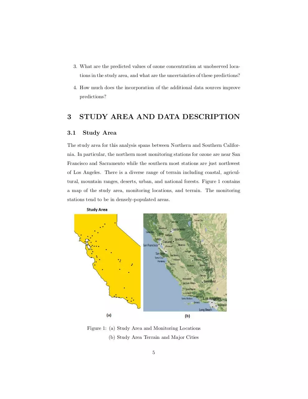
The study area for this analysis spans between Northern and Southern California. In particular, the northern most monitoring stations for ozone are near San
Francisco and Sacramento while the southern most stations are just northwest
of Los Angeles. There is a diverse range of terrain including coastal, agricultural, mountain ranges, deserts, urban, and national forests. Figure 1 contains
a map of the study area, monitoring locations, and terrain. The monitoring
stations tend to be in densely-populated areas.

Figure 1: (a) Study Area and Monitoring Locations
(b) Study Area Terrain and Major Cities
5

3.2
3.2.1

Data Description
Ozone monitoring

Ozone data for the analysis come from the EPA at the monitor level in the
form of an 8-hour average due to the fact that the national ambient air quality
standards (NAAQS) for ozone are in this form. That is, for every monitoring
station an 8-hour average is calculated for every clock hour. Only complete
data (e.g., with 6 or more valid hourly samples in the 8 hour block, or 75%
completeness) is included. The data are for the year 2015. The units for the
ozone measurements are in parts per million (ppm). The NAAQS for ozone is
that the annual fourth-highest daily maximum 8 hour average concentration,
averaged over 3 years can not exceed 0.070 ppm. Each observation is associated
with a latitude and longitude, date, etc.

• Dataset download link: http://aqsdr1.epa.gov/aqsweb/aqstmp/airdata/8hour 44201 2015.zip
• Codebook: http://aqsdr1.epa.gov/aqsweb/aqstmp/airdata/FileFormats.html# 8 hour average files
3.2.2

Elevation data

Elevation data for the analysis come from The Google Maps Elevation API,
which provides elevation data for all locations on the surface of the earth. In
those cases where Google does not possess exact elevation measurements at the
precise location you request, the service will interpolate and return an averaged
value using the four nearest locations. If the reader is interested in the API documentation, please visit https://developers.google.com/maps/documentation/elevation/intro.
3.2.3

Population density data

Population density (persons per square mile) data come from the 2010 Census
conducted by the U.S. Census Bureau at a “places” level (incorporated cities
and Census Designated Places). The ”2010 Census Summary File 1” dataset can
be downloaded directly from the American Fact Finder’s website. The location
6

of observations in the data is given by a character variable containing the city
or town name.
3.2.4

Meteorology data

Meteorology data come from the Weathersource.com API. Each query returns a
collection of weather history data for a given postal code. Specifically, average
cloud cover, average dew point, total precipitation, average relative humidity,
average surface pressure, average specific humidity, minimum temperature, average temperature, max temperature, and average wind speed are returned.
Unfortunately, the API restrictions limit users to 10 requests a minute, and
1000 per day. If the reader is interested in the API documentation, please visit
https://developer.weathersource.com/documentation/resources/get-history by postal code/.

4
4.1
4.1.1

METHODOLOGY
Data Preprocessing
Ozone data

First, the ozone dataset was subset only to observations in the study area. Next,
a decision was made to only use the 8-hour average from 8a.m. to 4p.m. This
seemed reasonable as it accounts for most of the sunlight during each day and
simplified the analysis. Finally, the data was subset to observations in August
for reasons mentioned in section 4.1.4.
4.1.2

Elevation data

The Google Maps Elevation API allows location requests in the form of a latitude and longitude pair. Thus, for every unique pair of latitudes and longitudes
in the ozone data, a request was made to the API and the elevation value was
extracted from the returned JSON object.

7

4.1.3

Population density data

To obtain population density data at every monitoring station, first a script was
written to get the city or town name at each monitoring station location. At
four percent of locations, a town or city name could not be identified and thus
observations with these locations were deleted. For each remaining location,
the observation in the population density dataset that had the corresponding
town/city name was found and the population density value for that observation
was integrated into the valid locations dataset. There were two special cases
when performing this integration. Some observations had a city name that
appeared in more than one row of the population density data. In this situation,
the observation with the highest total population count was used. The second
special case was for observations whose city name didn’t appear at all in the
population density data. This was a very small percentage and thus observations
with these locations were deleted.
4.1.4

Meteorology data

The meteorology API restrictions (10 requests per minute, 1000 requests per
day) made an analysis for all of 2015 infeasible in the time frame of this research.
Thus, the scope was reduced down to August as this is a hot summer month
where significant levels of ozone should be occurring. Since the meteorology
API accepts request for locations in terms of their zip code, a script was written
to obtain the zip code of each unique ozone monitoring station. Then, the
meteorology data was integrated as time permitted. Lastly, near-zero variance
meteorology predictors were removed (precipitation) as were highly-correlated
variables. Specific humidity was used instead of relative humidity and dew
point average. Average temperature was used instead of minimum or maximum
temperature.

8

4.1.5

Data integration for prediction locations

For making predictions, a grid of 265 latitude and longitude pairs was created
in the study area. The ideal number of prediction locations would have been
in the thousands, but due to the meteorology API restrictions the number 265
was chosen as a trade-off for the number of days the data would be able to be
collected in time. Then, the exact same data preprocessing/integration scripts
and methods were used on these new locations.

4.2
4.2.1

Exploratory Data Analysis
General

EDA and quantification of the data were handled by quantile summaries, histograms, box plots, scatter plots, etc. Geostatistical models assume a normal
distribution of the response variable at each monitoring station, and thus the
ozone values for each station for all 31 days were collected separately and the
Shapiro-Wilk normality test was performed on each. Approximately 44% of the
stations didn’t pass the normality test, and thus a new variable containing the
log transform of the ozone values was created for each dataset.
4.2.2

Variograms

Variograms are an exploratory tool used to describe the degree of spatial dependence and/or estimate the covariance parameters in a geostatistical model.
Formally, the theoretical variogram is defined as:

2Υ(h) = E[(Y (x) − Y (x + h))2 ]
Where x is a vector ∈ <2 of spatial locations, Y (x) is some quantity (in this case
8-hour ozone average in parts per million) available at all spatial locations, and h
is the lag distance between the pairs of locations. Υ itself is the semivariogram.
The empirical variogram (from the observed data) is an unbiased estimator of
the theoretical variogram and is defined as:
9