07 13Oct15 522 961 1 ED (PDF)

Bulletin of Electrical Engineering and Informatics
ISSN: 2302-9285
Vol. 5, No. 1, March 2016, pp. 62~71, DOI: 10.11591/eei.v5i1.522



62

Basis Weight Gain Tuning Using Different Types of
Conventional Controllers
Chandani Sharma*1, Anamika Jain2
Electronics and Communication Engg. Dept. Graphic Era University, Dehradun Uttrakhand, India
*Corrresponding author, e-mail: chandani19nov@gmail.com1, anamikajain2829@gmail.com2

Abstract
Paper making is a vast, multidisciplinary technology that has expanded tremendously in recent
years approaching to reach 20 million tons by 2020. As per demand implementation of necessary tools to
optimize papermaking process and to increase the control precision, the precondition for stable operation
and quality production is necessary. In the present work, an effort has been made to analyse gain tuning of
Basis Weight output relative to the changing values of basis weight valve opening with step and variable
input. The effects of the three constants KP, KD and KI for different types of conventional controllers as P,
PD and PID controller are examined by adding a disturbance to the control system. The effects of various
scaling gains are studied on the output of the system and are tuned to get the optimum output both for the
step input as well as the varying input. Simulation results show that P, PD and PID controllers provide
automatic tuning to preserve good performance for various operating conditions. An analysis of practical
performance indices is presented by comparing results of three different conventional controllers. The
system developed can be used to serve as platform for Control engineering techniques used in industries.
Keywords: KP, KD and KI Conventional, P, PD and PID controller, scaling gain, automatic tuning

1. Introduction
The Indian Paper Industry accounts for about 1.6% of the world’s production of paper
and paperboard. Paper Industry in India is moving up with a strong demand push and is in
expansion mode to meet the projected demand. The main requirement for industries today is
that, the companies must be more productive, flexible and produce high quality goods for
customers and market requirements in the world market’s conditions [1]. Therefore, every stage
in organization and production systems can be used for continuous improvement. For this
purpose, many tools, techniques, subsystems and systems can be used.
The papermaking process is a very complicated process with varying; heat and mass
transfer steps at different stages. Paper machine controls try to keep quality variables at their
target levels with minimum variability. Each paper grade has its specific targets and limits for
many quality variables such as Basis weight, Moisture, Caliper, Ash content, smoothness,
Gloss, Formation, strength properties, Fault distribution etc. Out of these, Basis weight and
moisture content are the two important parameters of quality which are measured and controlled
on line [2], [3].

2. Basis Weight
The grammage per square meter (GSM) is considered as the target end product of
paper. It not only reflects the quality of the end product, but also affects the economy. Therefore
it must be controlled. The primary factor influencing the basis weight is the pulp flow that can be
controlled by the basis weight valve opening at the head box. Thus the process as a whole has
one controlled output i.e. Basis weight (B) and one manipulated input i.e. pulp flow (G)
monitored by the basis weight valve opening (BWVO) at the head box. The input-output
relationship is given by equation (1.1) that relates Transfer function between input function
"G(s)" to output function “B(s)” [4]. It is given by:

Received September 23, 2015; Revised November 13, 2015; Accepted December 8, 2015

63

ISSN: 2089-3191


B(s)
5.12
------ = exp (-144*s) ----------G(s)
105 s + 1

(1)

Where
G(s) = Pulp Flow at head box
B(s) = Basis weight per square meter
Exp (-144*s) = Transportation Lag
105 = τ time constant of system in seconds
5.12= K constant representing the dimensional conversion factor based on equipments
involved in the system.
The basis weight is continuously measured online on the reel and any variation required
in its set point is accordingly adjusted by varying the basis weight valve opening at the head
box. The data for basis weight has been collected from a middle density basis weight mill,
where the speed of the paper machine is around 250 m/min and length of paper traveled from
the head box to the reel is approximately 600 meters.

3. PID Controllers
PID controller is one of the earliest industrial controllers. A proportional-integralderivative controller (PID controller) is a controlled closed loop feedback system that calculates
an error value as the difference between a measured process variable and a desired set point.
The controller attempts to minimize the error by adjusting the process through use of a
manipulated variable. It has many advantages of being robust, economic, simple and easy to be
tuned. However, in spite of these advantages of the PID controller, there remain several
drawbacks [5], [6]. It cannot cope well in cases of Non-linear time varying processes,
compensation of rapid disturbances, and supervision in multivariable control.
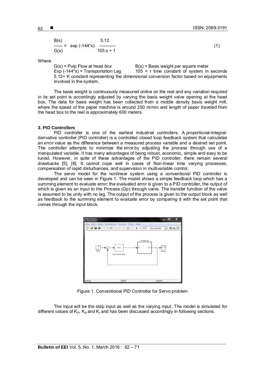
The servo model for the nonlinear system using a conventional PID controller is
developed and can be seen in Figure 1. The model shows a simple feedback loop which has a
summing element to evaluate error; the evaluated error is given to a PID controller, the output of
which is given as an input to the Process (Gp) through valve. The transfer function of the valve
is assumed to be unity with no lag. The output of the process is given to the output block as well
as feedback to the summing element to evaluate error by comparing it with the set point that
comes through the input block.

Figure 1. Conventional PID Controller for Servo problem
The input will be the step input as well as the varying input. The model is simulated for
different values of KP, KD and KI and has been discussed accordingly in following sections.

Bulletin of EEI Vol. 5, No. 1, March 2016 : 62 – 71

Bulletin of EEI

ISSN: 2302-9285



64

4. Servo Model for Step Input
(a) P Type Controller
In this case, only the Proportional gain constant i.e. KP is given some specified value
and the other two gains i.e. the differential (KD) and integral (KI) gains are kept at zero. Different
values are assigned to KP while KD and KI were kept zero. It was found that for a step input, on
increasing the value of KP, the system response became more and more oscillatory and hence
the system became unstable. Simulation results for test done for KP = 0.1, 0.2, 0.3 and 0.5 can
be seen in the Figure 2. It is clear that the system becomes unstable at KP = 0.5. It is also
observed that though the oscillatory behavior increases with the increase in KP but the offset is
also reduced to some extent.

Figure 2. Output for step input servo model for the basis weight for varying values of KP
Again tests were performed for some more values of KP, to find the out optimum value of KP for
the step input of the system. Now the test values were taken as KP = 0.3, 0.32, 0.34, 0.38. The
simulation results for the same are plotted in Figure 3.

Figure 3. Output for step input servo model for the basis weight for varying values of KP
It is observed from Figure 3 that for values of KP equal to and below 0.38, the system
gives the bounded output and hence it is stable though very oscillatory. But as can be seen in
the next simulation result (Figure 4) that as the value of KP increases beyond 0.4 the system
suddenly becomes unstable. The simulation results for different values of KP = 0.35, 0.38, 0.4,
0.42 are shown in Figure 4.

Basis Weight Gain Tuning Using Different Types of Conventional Controllers (Chandani S)

65



ISSN: 2089-3191

Figure 4. Output for step input servo model for the basis weight for varying values of KP
Out of all these test values, KP = 0.1 was selected as the optimum value as it had the
minimum oscillatory behavior.
(b) PD Type Controller
Once the value of KP has been selected, now the system is tuned for optimum value of
KD. As it is a PD type of controller, therefore KI is kept zero. Thus the simulation is performed for
KP as 0.1 and KI as zero and different values of KD are taken as 0.1, 1, 10, and 20, the results
for the same can be seen in the Figure 5.

Figure 5. Output for step input servo model for the basis weight for varying values of KD
It can be clearly seen from Figure 5 that as the value of KD increases the overshoot is
decreased i.e. the derivative action dampens the system and tries to improve the stability of the
system, though for higher values of KD the response is oscillatory but yet stable. Tests are also
performed for KD = 0.001, 0.01, 0.1 and the results for all the three values were almost
coinciding. Thus out of all these values KD = 0.1 gives the best results; hence it is taken as the
optimum value. It can be said here that the value of KD if increased to a large extent affects the
system output, for smaller values of KD the output has minor affect on its dynamics.
(c) PID Type Controller
Now the effect of integral part is analyzed by introducing the KI part in the system. The
optimum values of KP and KD are taken from the above results. KP = 0.1 and KD = 0.1 is taken
and Different values of KI are taken as KI = 0.001, 0.0005, 0.0001, 0.00001. The results for the
same can be seen in Figure 6.

Bulletin of EEI Vol. 5, No. 1, March 2016 : 62 – 71

Bulletin of EEI

ISSN: 2302-9285



66

Figure 6. Output for step input servo model for the basis weight for different values of KI
It can be seen from Figure that as the value of KI increases, the offset is decreased.
For KI = 0.001, the offset is zero, even for KI = 0.0005 the offset is zero. But for the values of KI
above this, the offset appears. Tuning of the system becomes difficult; hence the tests are again
performed for values of KI between 0.0005 and 0.001. The simulation results are shown in
Figure 7 for other values i.e. for KI = 0.0006, 0.0007, 0.0008 and 0.0009, KP = 0.1and KD = 0.1.

Figure 7. Output for step input servo model for the basis weight for varying values of KI
It is clear from Figure 7 that the value of KI between 0.0007 and 0.0008 would give the
optimum value. Tests were done and the value of KI = 0.00073 which gave a minimum
overshoot and zero offset was taken as the optimum value. Also it is observed that the integral
part is responsible for the offset and also the overshoot for servo model with step input. Thus a
conventional controller with an optimum output for the step input-servo model has been
developed with values for different gains as: KP =0. 1, KI = 0.00073, KD = 0.1.
The model of Figure 1 using a PID controller is simulated for variable inputs i.e. the data
for the reference inputs is collected from the mill where online sensors are incorporated and the
value of the inputs. Thus the basis weight continuously changes according to the demand. This
data has been saved in the m-file of Matlab and is collected from the workspace from where it is
given as the input to model of Figure 1. First a P-Type controller is made to run and then further
PD and then PID models are simulated.

Basis Weight Gain Tuning Using Different Types of Conventional Controllers (Chandani S)

67



ISSN: 2089-3191

5. Servo Model for Varying Input
(a) P Type Controller
Different values are assigned to KP, the Proportional gain and the other two gains i.e.
the integral (KI) and the differential (KD) gains are kept at zero. Thus the different values
assigned to the gains are KD=0, KI=0 and different values of KP are KP = 0.1, 0.2, 0.3, and 0.4 as
in Figure 8.

Figure 8. Output for varying input servo model for basis weight for varying values of KP
It can be seen from Figure 8 that as the value of KP increases the response of the
system becomes more and more oscillatory, but it is also clear from the response that the effect
of change in the values of the reference input on the output response is almost nil for different
values of KP. Thus the system response is very poor. Moreover it is also seen that as the value
of KP is increased beyond 0.4 the system becomes highly unstable. For KP = 1 the Y- axis
becomes 1× 1010. So from the above results the optimum value of KP is selected as 0.1 for
further work.
(b) PD Type Controller
To behave like a PD-Type of Controller, the term KD is assigned some value in servo
model instead of zero. Now KP = 0.1, and KI = 0 and different values of KD are taken as: KD=1,
0.1, 0.01 and 0.001. As seen from the simulation result shown in Figure 9 that the output of all
the values of KD almost coincide. A minor difference is seen in the overshoot but rest curves are
almost the same for all values.

Figure 9. Output for varying input servo model for basis weight at different values of KD
Bulletin of EEI Vol. 5, No. 1, March 2016 : 62 – 71

Bulletin of EEI

ISSN: 2302-9285



68

Simulation is again performed for more values of KD such as KD = 1, 10, 15 and 20
keeping KP = 0.1, and KI = 0, and it was observed that as the value of KD is increased, the
oscillatory behavior increases as can be seen in Figure 10 but there is no effect of changing
input on any of these values. The system output does not vary according to the Basis weight
and set point changes. Thus from the above results the value of KD =1 is taken as the optimum
value.

Figure 10 Output for varying input servo model for basis weight for varying values of KD
(c) PID Type Controller
The integral term KI term is introduced to the servo model. The simulation was
performed for various values of KI as in Figures 11, 12 and 13. The different values of KI in
Figure 11 are 0.00005, 0.00001, 0.000005, and 0.000001 while the values of KP and KD are
taken as 0.1 and 1 respectively. It is clear that the response for all the values does not vary with
the changing input. Also it is observed that as the value of KI increases, the offset is reduced to
some extent.

Figure 11. Output for varying input servo model for basis weight for varying values of KI
The simulation is performed for more values of KI as 0.0005, 0.0001, 0.00007, and
0.00001 while KP and KD are taken as 0.1 and 1 respectively. For these values in Figure 12
same observations are made as above i.e. as the value of KI increases, the offset is reduced.

Basis Weight Gain Tuning Using Different Types of Conventional Controllers (Chandani S)

69



ISSN: 2089-3191

Figure 12. Output for varying input servo model for the basis weight for varying values of KI
It has been observed from the simulation results that for none of the values of KI, the
system is giving a good output. The system is giving a bounded output for some values but as
the value of KI is increased beyond 0.001, the output becomes quite unstable. The same can be
seen in the scope window of Figure 13. where different values of KI are taken as KI = 0.005,
0.001, 0.0007 and 0.0001, keeping the value of KD and KP same as for the above cases.
Moreover for none of the cases the output is changing along with the input hence the system
response is very poor.

Figure 13. Output for varying input- servo model for the basis weight when the value of KI is
0.001
It is worth mentioning here that as the value of KI increases beyond 0.001, the system
becomes unstable, as it gives the unbounded output for the bounded input.

6. Results and Analysis
An ideal proportional controller, with increase in value of KP decreases rise time but
does not eliminate the steady state error. An integral control Ki eliminates steady state error but
makes response slower. A derivative control Kd increases stability, reduces over shoot, and
improves response. Table 1 [11] highlights the effect of different parameters on ideal
proportional controller. Table 2 gives the outputs relative to basis weight step and variable input
experiments.

Bulletin of EEI Vol. 5, No. 1, March 2016 : 62 – 71

ISSN: 2302-9285

Bulletin of EEI



70

Table 1. Ideal Proportional Controller Time, Overshoot and Error
CONSTANT

RISE TIME

OVER SHOOT

SETTLING TIME

STEADY STATE ERROR

Kp

Decrease

Increase

Small Change

Decrease

Ki

Decrease

Increase

Increase

Eliminate

Kd

Small change

Decrease

Decrease

No Change

Table 2. Basis weight Closed loop Time, Overshoot and Error
CONSTANT

RISE TIME

OVER SHOOT

SETTLING TIME

STEADY STATE ERROR

Kp
Ki

Decrease

Increase

Small Change

Decrease

Increase

Decrease

Increase

Kd

eliminate

Small change

Decrease

Decrease

No Change

It is clear that increase in Ki produces opposite effect when compared to conventional
controllers. Similarly for both step input and variable input, the value of KP responsible for offset
as well as the oscillatory behavior is tabulated in Tables 3 and 4.
Table 3. Ideal Closed loop Stability, Accuracy and Response
CONSTANT

STABLITY

ACCURACY

RESPONSE TIME

Kp

Deteriorate

Improve

Increases

Ki

Deteriorate

Improve

Decrease

Kd

Improve

No impact

Increases

Table 4. Basis weight Closed loop Stability, Accuracy and Response
CONSTANT

STABLITY

ACCURACY

RESPONSE TIME

Kp

Improve

Improve

Increases

Ki

Deteriorate

Improve

Decrease

Kd

Improve

No impact

Increases

If offset has to be reduced the value of KP has to be increased but it results in increase
of oscillations in the system. While relating distinction of step input and variable input oscillatory
effect was higher for variable values of basis weight as compared to step input. Talking about
value of KD, an increase in its value decreases the overshoot i.e. the derivative action dampens
the system and tries to improve the stability of the system. Though, for higher values of KD
response is oscillatory, yet stable. It can be indicated from the results that decreasing KI causes
offset to appear in the system and vice versa.
Based on different Controllers, it is described that Proportional controller accelerates
response, but has a non-zero offset making system unstable. PD controller causes damped
oscillations leaving offset but results increase in stability. In PID controller, integral action
eliminates offset oscillations.

7. Conclusion and Future Scope
Servo control responds to change in set point. There could be improved model design
consideration as regulatory control. It responds to a change in some input value, bringing
system in steady state. FLC based systems can be designed in the process industries for such
case studies.

Basis Weight Gain Tuning Using Different Types of Conventional Controllers (Chandani S)