KMeansRE (PDF)

C#.NET Implementation of K-Means Clustering Algorithm to Produce
Recommendations.
“K-means is a widely used method in cluster analysis. In my understanding, this method does NOT
require ANY assumptions, i.e., give me a data set and a pre-specified number of clusters, k, then I just
apply this algorithm which minimize the SSE, the within cluster square error.” – David Robinson, Data
Scientist at StackOverflow.

Introduction
K-Means clustering is one of the most reliable unsupervised learning data mining algorithms used as a
workaround to the famous clustering problem that had previously been considered to be noncomputational. The following algorithm was initially proposed by Hugo Steinhaus and Stewart Lloyd in
1950 and improved by James McQueen in 1967. Since that time, K-means clustering algorithm is used to
solve a variety of computational problems such as sum of squares error (SSE) minimization in regression
analysis, graphical image segmentation, recommender engines development, maintaining efficient
software features that provide public safety over the Internet and anti-theft protection, etc.
In this article, we’ll discuss about how to use K-means clustering algorithm to implement a simple
recommender engine that performs user-to-item collaborative filtering to recommend articles published
in a certain social media website to a community of users according to their personal preferences.

Background
In this section of the following article we’ll provide an understanding of the very basic representation of
the classical k-means clustering algorithm used to solve many computational problems. In particular, we’ll
thoroughly discuss about the essentials of the k-means clustering procedure as well as

K-Means Clustering Algorithm Fundamentals
In general, k-means algorithm provides a solution to the trivial classification problem by splitting up a
certain dataset into k - clusters, each one containing a number of the most similar data items (or just
“observations”) arranged into a cluster based on a minima distance to the nearest “mean”, which, in turn,
is being a “prototype” of the following cluster. In the other words, k-means clustering algorithm selects
n items from the entire dataset that have a closest distance to a particular nearest mean and builds a
new cluster. According to the following algorithm, k-means procedure selects the number of the most
similar items for each nearest mean, the value of which is previously computed for each particular new
cluster being created.
In this case, for each nearest mean’s value we’re performing a computation of a separate cluster
containing those data items that are the most similar to the current nearest mean. Another important
condition of the clustering process is that each item being selected by k-means procedure from the given
dataset must have the closest distance (e.g. must be the most similar) to the other items included in the
same cluster. The main idea of performing k-means clustering is that if two different items being selected
have the minima distance (i.e. similarity) to the same nearest mean, then the actual distance between
these items also tends to the minima.
The value of each item in the given dataset is basically represented by a set of attributes that describe the
following item. The set of attributes for the given item normally has a numerical representation, in which
each attribute is a real value. That’s why, the entire set of attributes associated with a data item is denoted
as a certain vector I  {i0 , i1 , i2 ,...,in1 , in } in n - dimensional Euclidean space, where n is an actual
number of attributes that describes the data item ( I  R n ).

In turn, the value of the nearest mean computed for each new cluster is also represented as a numerical
real vector of attributes C  {c0 , c1 , c2 ,...,cn1 , cn } having a particular distance to the vector of attributes

I for each item in the n - dimensional Euclidean space. Actually, the vector of attributes C for a certain
nearest mean, contains those attributes which values are the most common to each item in the cluster.
As we’ve already mentioned above, the nearest mean, itself, provides a generalization for a certain
number of items being selected into a cluster, and serves as a prototype of the entire cluster. For example,
if we have two items belonging to the same cluster and each one having a certain vector of attributes I t
, then the vector of attributes C , associated with the nearest mean for these two items, would consist of
those values that have a closest distance to the values of attributes that are contained in both vectors for
one item and another item respectively.
The distance between a particular data item in the given dataset and the nearest mean is computed by
using an objective function, such as Euclidean, Manhattan or Taxicab distance, which value normally
represents similarity between an item and the nearest mean based on the distance between the vectors
of attributes of either the nearest mean C or a particular item I t in a cluster. According to the k-means
clustering algorithm it’s the most preferable to use Euclidean distance function rather than the other
functions that allow to compute the following distance. The Euclidean distance is normally computed as
a sum of squares of partial distances between particular attributes that describe the nearest mean and
an item, and can be formulated as follows:
NP

d 2 (C, I t )   (in(t )  cn ) 2

(1)

n1

, where d 2 (C, I t ) - the distance between two vector of attributes of either the nearest mean C and an
item I t in a cluster; in(t ) - the value of attribute n of the item t ; c n - the value of attribute n of the current
nearest mean; N P - the actual number of attributes;
Basically, there’s a variety of methods by using which we can compute the nearest mean’s vector of
attributes C for each particular cluster. In the most cases, the nearest mean’s attributes vector is
computed as the vector that represents a center of mass for a certain subset of items. The following center
of mass is also called a “centroid” of a newly built cluster. Particularly, the centroid’s vector of attributes
is obtained by computing an average (“mean”) of attribute values of all items within a cluster. In order to
compute the average vector of attributes, we actually need to perform by-component addition of multiple
vectors of attributes associated with the all items in a cluster. The following formula illustrates the
computation of a single centroid’s attribute value c n which is a component of vector C for the given
centroid:

cn 

1 N I (t )
  in
N I t 1

(2)

, where c n - the value of attribute n in the vector of attributes for the given centroid; in(t ) - the value of
attribute n of the item t ; N I - the actual number of items in a cluster;
Generally, the step-by-step k-means clustering procedure can be formulated as follows:
0. Build an initial cluster from the entire dataset of items: Before we begin we need to assign all
items in the given dataset to an initial cluster and append it to the array of clusters. Also we’ll
have to select a set of multiple centroids for the initial cluster. Notice that, unlike the other

succeeding new clusters that will be further produced by the k-means procedure, to perform an
efficient clustering, the initial cluster should contain more than one centroid;
1. Randomly initialize k centroids of the initial cluster by using the either Forgy or Random
Partition methods: To perform initialization we actually have to generate a vector of attributes
for each current centroid i  1, k by assigning random values to each attribute cn(i ) , n  1, N P
of the vector Ci . Also, at this step, we assign the initial values to the loop counter variables

q  0 and i  0 ;
2. For the current cluster q retrieved from the array of clusters find the items with the minima
distance to each centroid i and produce the new clusters: During this step we retrieve a cluster
from the array and proceed with the next steps to create one or more new clusters based on the
set of centroids belonging to the current cluster;
3. For the current centroid i , compute the actual distance to each item t by using Euclidean
distance formula (1): At this point we need to compute the distances between the vector of
attributes Ci associated with the current centroid i and the vector of attributes I t for each
item;
4. Choose n items having the closest distance to the current centroid i and produce a new
cluster by assigning each item with the minima distance to the newly created cluster: To do
n

this, we basically use the following formula arg min{d t2 (Ci , I t )}to find all items with vector of
t

attributes I t that satisfies the minima distance criteria to the current centroid’s i vector of
attributes Ci ;
5. Compute the new value of centroid based on the formula (2) and assign it to the new cluster
produced at the step 4: During this essential step we will compute the new centroid’s vector of
attributes Ci1 as a center of mass represented as a by-component vectors of attributes I t ,
summation for each item t  1, N I contained within the newly built cluster. After that, we’ll
assign the new centroid to the following cluster. In case, if we cannot compute the new value of
centroid for the new cluster, go to the next step of the algorithm, otherwise proceed with step
7;
6. Output the newly built cluster: At this point we assume that there’s no more clustering possible
for that particular cluster. That’s why, we pass the following cluster to the output. Similarly,
we’ll perform the output for each new cluster that exactly meets the condition applied in the
previous step 5. After we’ve produced the output, go to step 8 and proceed with the next
centroid (i  1) ;
7. Append the new cluster obtained at the previous steps to the array of clusters and proceed
with the next step of the following algorithm: At this step we will insert the new cluster
obtained into the array of clusters, which is basically used as clusters queue while performing
the recursive clustering, during which, each one cluster in the array is separated into the number
of new clusters based on the values of one or many of its centroids. Finally, we proceed with the
next step of the algorithm;
8. Select the next centroid (i  1) for which we’ll be performing the actual clustering, and
perform a check if this is the final centroid of the current cluster ( i  N M  1 ) retrieved from
the array of clusters: If so, proceed with the step 9, otherwise perform steps 3-7 to produce the
rest of new clusters for each centroid of the current cluster;
9. Select the next cluster (q  1) from the array of clusters and perform the check if this is the
final cluster in the clusters queue ( q  N C  1 ) or there’s no ability to re-compute the new

centroid for the currently processed cluster: If so, terminate the k-means clustering process,
otherwise return to the step 2;
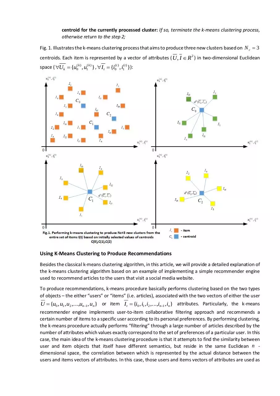
Fig. 1. Illustrates the k-means clustering process that aims to produce three new clusters based on N c  3
centroids. Each item is represented by a vector of attributes ( U , I  R2 ) in two-dimensional Euclidean
space ( U k  {u0( k ) , u1( k ) } , I t  {i0(t ) , i1(t ) }):

Using K-Means Clustering to Produce Recommendations
Besides the classical k-means clustering algorithm, in this article, we will provide a detailed explanation of
the k-means clustering algorithm based on an example of implementing a simple recommender engine
used to recommend articles to the users that visit a social media website.
To produce recommendations, k-means procedure basically performs clustering based on the two types
of objects – the either “users” or “items” (i.e. articles), associated with the two vectors of either the user

U  {u0 , u1 , u2 ,...,un1 , un } or item I t  {i0 , i1 , i2 ,...,in1 , in } attributes. Particularly, the k-means
recommender engine implements user-to-item collaborative filtering approach and recommends a
certain number of items to a specific user according to its personal preferences. By performing clustering,
the k-means procedure actually performs “filtering” through a large number of articles described by the
number of attributes which values exactly correspond to the set of preferences of a particular user. In this
case, the main idea of the k-means clustering procedure is that it attempts to find the similarity between
user and item objects that itself have different semantics, but reside in the same Euclidean n dimensional space, the correlation between which is represented by the actual distance between the
users and items vectors of attributes. In this case, those users and items vectors of attributes are used as

sets of trivial latent parameters by using which we establish the relationship between the user and item
objects. In this case, the similarity measure, represented by the Euclidean distance between the either
user or item’s vector of attributes, is computed based on the most similar attributes (e.g. having the
closest distances between one another). In the other words, we actually obtain the similarity between
users and items by computing the sum of squares of partial distances between particular attributes. The
following process generally implies the either sum of squares error minimization (SSE) performed by using
the ordinary least squares (OLS) method in regression analysis, or singular value decomposition (SVD)
computation in latent sematic analysis, capable of providing the user-to-item recommendations.
To do this, k-means clustering algorithm aims to find the number of items that are the most similar to a
specific user having its own preferences represented by a vector of attributes U , and computes clusters
in which a specific user, associated with the number of items, serves as the nearest “mean” (or “centroid”)
of the entire cluster. In this particular case, the similarity of users and items is typically represented by
Euclidian distance (i.e. “metric”) between two vectors of both a user’s U and item’s I t attributes
respectively. For that purpose, we use slightly different formulas to perform the similarity computation:
NP
1

sw2 (U , I t )     (in(t )  un ) 2 
n 1  rn


(3)

, where sw2 (U , I t ) - the weighted measure of similarity value between a user and an item; in(t ) - the value
of attribute n of the item t ; u n - the value of attribute n for a specific user; rn - the coefficient of
relevance between attribute n of the user’s and item’s vectors of attributes; N P - the actual number of
attributes;
Unlike the conventional Euclidean distance formula that allows to compute the actual distance between
two vector of attributes, discussed above, the measure of similarity is obtained as a weighted distance
value represented as a sum of squares of partial distances between the either user’s or item’s particular
attributes, each one is multiplied by a specific weight coefficient rn . In this case we basically deal with the
distance-based similarity which value depends on the more than one parameter. A set of multiple extra
parameters of the following formula (3) is represented as a dividend that includes the sum of those extra
parameters for a specific attribute:

( n)
0

r

r

( n)
1

1
, where rv(n ) - is an extra
 r  ...  rv(n1)  rv( n)
( n)
2

parameter v of attribute n for a specific user or item.
In this case, besides the partial distance between user’s and item’s attributes we also use a single
parameter rn – the relevance between those attributes. Since we implement the contextual data model
to be used to produce recommendations, we will employ the measure of lexicographical relevance as the
parameter rn of the formula (3).

 1
rn   
j  min{L}


i (j n )  u (jn ) 


(4)

)
, where rn - the value of lexicographical relevance between attribute n of a specific user and item; i (n
j )
the character j in the string representation of attribute n of a specific item; u (n
j - the character j in the

string representation of attribute n of a specific user; min{L} - the actual length of the smallest of two
strings that represent the either user or item attribute n ;

To compute the relevance of the either user or item attributes, we normally use a trivial linear search
algorithm by iterating over the two strings that represent attribute n and for each position we’re
)
(n )
performing the comparison of characters located at the same position j . If those characters u (n
j and i j

exactly match, then we add the value of

1
to the totally estimated value of the relevance rn . The
L

parameter L is the actual length of the smallest string the represent the either user’s or item’s attribute
n . The more about the lexicographical representation of users and items attributes as an essential part
of contextual data representation model is discussed in the next section of the following article.
Also, to provide more flexible distance-based similarity computation using formulas (3,4), it’s
recommended to modify formula (3) by using another extra parameter, that represents the actual number
of either user’s or item’s attributes m that exactly match having the value of relevance rv( n)  1 . The
main reason why we use the following parameter in formula (3) is that the similarity of specific users and
items, represented by the value of actual distance between the either user’s or item’s vector of attributes,
largely depends on the number of attributes that are lexicographically equal. In this case, formula (3) has
the following representation:

sw (U , I t ) 

1

m

NP

1

n 1



r

n


 (in(t )  un ) 2 


(5)

A large number of attributes that lexicographically match ensures that the Euclidean distance between
the two vectors of either user’s and item’s attributes is typically small and obviously the measure of
similarity between a specific user and item normally grows. However, there’s a special case when a
specific user and item selected are merely dissimilar (e.g. the either vectors of user’s or item’s attributes
don’t have any attributes that exactly match) and the value of extra parameter m  0 . In this case, we
assume the value of parameter m to be equal to 0.01, which means that the actual distance between the
either user’s or item’s vector of attributes tends to be large. In the other words, we use the value of
parameter m  0.01, which in turn provides a typically large distance between dissimilar user and item
to avoid the case in which the most dissimilar items have a closer distance to a specific user rather than
the other of items having a greater value of distance-based similarity compared to any of existing
dissimilar items.
In the next section of this article, we’ll make a focus on the basic representation of each particular article
and user as an essential part of the contextual data model used by the K-means clustering procedure to
produce recommendations.

K-Means Clustering and Contextual Data Model
According to the contextual data model, each item is represented by a string of characters containing a
title of a particular article published in social media. Obviously that, the following string consists of the
number of “keywords” delimited by a space-character. Also each item is associated with a set of attributes
that describe the following item. Each attribute assigned to an item has a string representation and is
treated as a “keyword” that describes a user or item. Normally, we determine the user-to-item distancebased similarity based on the similarity of particular attributes being encoded and assigned to a user or
item. In the first case, each attribute assigned to an item exactly describes the either contents of an article
or the category to which the following article belongs. In the other case, the set of user’s attributes
describes the personal preferences of each particular user. To represent a user or item within the
contextual data model we basically deal with two types of attributes: attributes that have been assigned
to a user or item as well as the attributes obtained as the result of extracting of each “keyword” from the
title of an article. In this case, both types of item’s attributes are represented as an entire set of attributes

associated with an item. The main difference between a user’s and item’s attributes representation is that
the set of attributes of each user, for which we’re performing search to find the most similar items,
normally don’t include the attributes obtained as the result of parsing a title of a specific user. In the other
words, by processing the data on each particular user we don’t parse its title. The set of attributes for
each particular user contains only those attributes that were previously assigned to a user.
In this case, we initially assume that each keyword is a lexicographical representation of a particular
attribute that describes an item as it’s shown in Fig. 2.:

In this case, each user or item is denoted as a certain vector of attributes, in which each attribute has the
either lexicographical or numerical representation. In particular, as you can see from Fig. 2 each
“keyword” delimited by a space-character is treated as a specific attribute of the given item. Further, the
string value of an item’s t attribute n is encoded as a numerical value in(t ) and used by the k-mean
clustering procedure to determine the similarity between particular user and item. Similarly, users that
serve as centroids for the following clustering process, are also represented as a set of string attributes,
each one having a numerical representation un(k ) . According to the contextual data model used along with
the k-means clustering process to produce recommendations, both a user’s and an item’s attributes are
encoded into the two vectors of attributes U k and I t for each particular item. The main reason why
particular attributes are encoded into the numerical values and are represented as a real vector of
attributes is that, according to the k-mean clustering algorithm we normally compute the similarity
between particular users and items by using Euclidean distance formula that basically deals with
numerical real vectors that reside in n - dimensional Euclidean space. From the other respect we use the
numerical representation of either users and items attributes, since it’s very hard to determine the actual
value of similarity between particular attributes based solely on a string representation of a user or an
item. There’re basically two main conditions under which we can actually compute the similarity of a user
and item. The first condition is that to compute the similarity between particular attributes n of either
user or item’s vectors of attributes it’s necessary that both attributes should belong to the same
geometrical plane within the n dimensional Euclidean space. In the other words, we can only compute
the distance between those attributes that are located and encoded at the same position n in the given
pair of vectors of attributes. For example, as it has been shown in Fig. 2., both user U k and item I t contain
the keyword “POSIX” that further will be encoded into a specific value of attribute. Unfortunately, the
following keyword located in the different position in either user or item set of attributes. That’s actually
why, before computing the actual distance between similar attributes we transform the either vectors of
attributes, so that the following attribute i5(t ) is located at the same position 1 in both user’s and item’s

vectors of attributes by exchanging the attribute i5(t ) with the attribute i1( t ) in the item’s vector of
attributes. Another important condition being applied is that the relevance of both a user’s i1( t ) and item’s

u1( k ) attributes must tend to the maximum. In this case, the string values of both user’s and item’s
attributes at the position n  1 are equal, which means that the following attributes i1( t ) and u1( k ) have
the maximum possible relevance, which is equal to r1  1.00 .