chapter 23 (PDF)

Chapter 23
1. THINK This exercise deals with electric flux through a square surface.



EXPRESS The vector area A and the electric field E are shown on the diagram below.

The electric flux through the surface is given by   E  A  EA cos .



EXPRESS The angle  between A and E is 180° – 35° = 145°, so the electric flux
through the area is





  EA cos   1800 N C  3.2 103 m cos145  1.5 102 N  m2 C.
2



LEARN The flux is a maximum when A and E points in the same direction (   0 ),
and is zero when the two vectors are perpendicular to each other (   90 ).
 
2. We use   E  dA and note that the side length of the cube is (3.0 m–1.0 m) = 2.0 m.

z

(a) On the top face of the cube y = 2.0 m and dA   dA ˆj . Therefore, we have





2
E  4iˆ  3  2.0   2 ˆj  4iˆ  18jˆ . Thus the flux is



top

E  dA  

top

 4iˆ 18jˆ   dA ˆj  18

top

dA   18 2.0  N  m2 C  72 N  m2 C.
2


(b) On the bottom face of the cube y = 0 and dA  dA  j . Therefore, we have

c

b ge j

h

E  4i  3 02  2 j  4i  6j . Thus, the flux is



bottom

E  dA  

bottom

 4iˆ  6jˆ   dA  ˆj  6

bottom

1040

dA  6  2.0  N  m2 C  24 N  m2 C.
2

1041

 

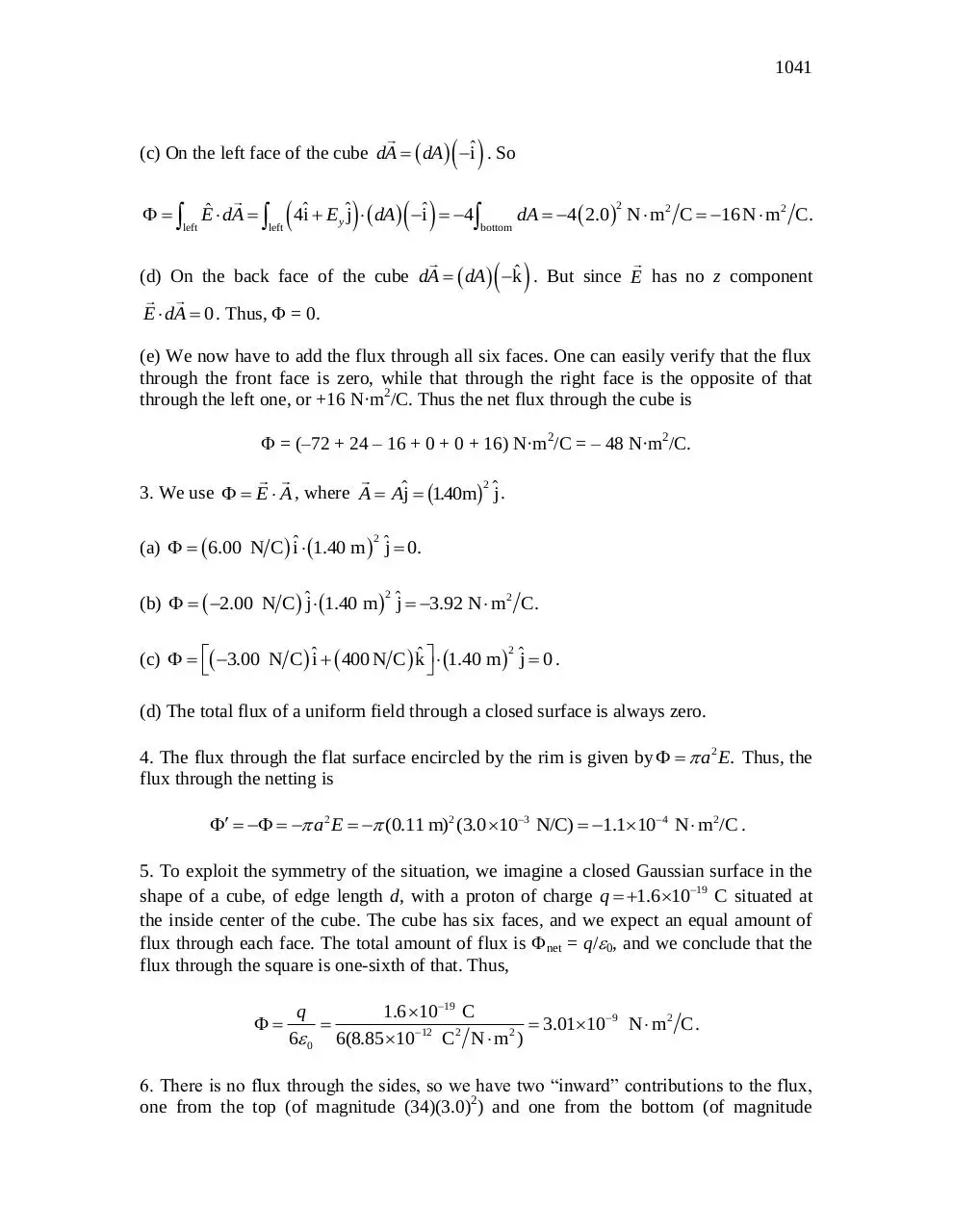
(c) On the left face of the cube dA   dA ˆi . So

   Eˆ  dA  
left

left

 4iˆ  E ˆj   dA  ˆi   4
y

dA  4  2.0  N  m2 C  16 N  m2 C.
2

bottom

 

(d) On the back face of the cube dA   dA kˆ . But since E has no z component

E  dA  0 . Thus,  = 0.
(e) We now have to add the flux through all six faces. One can easily verify that the flux
through the front face is zero, while that through the right face is the opposite of that
through the left one, or +16 N·m2/C. Thus the net flux through the cube is
 = (–72 + 24 – 16 + 0 + 0 + 16) N·m2/C = – 48 N·m2/C.


 
2
3. We use   E  A , where A  Aj  140
. m j .

b

g

2
(a)    6.00 N C  ˆi  1.40 m  ˆj  0.

2
(b)    2.00 N C  ˆj  1.40 m  ˆj  3.92 N  m2 C.

2
(c)    3.00 N C  ˆi   400 N C  kˆ   1.40 m  ˆj  0 .



(d) The total flux of a uniform field through a closed surface is always zero.
4. The flux through the flat surface encircled by the rim is given by    a 2 E. Thus, the
flux through the netting is
     a E   (0.11 m)2 (3.0 103 N/C)  1.1104 N  m2 /C .

5. To exploit the symmetry of the situation, we imagine a closed Gaussian surface in the
shape of a cube, of edge length d, with a proton of charge q  1.6 1019 C situated at
the inside center of the cube. The cube has six faces, and we expect an equal amount of
flux through each face. The total amount of flux is net = q/0, and we conclude that the
flux through the square is one-sixth of that. Thus,


q
1.6 1019 C

 3.01109 N  m2 C.
6 0 6(8.85 1012 C2 N  m 2 )

6. There is no flux through the sides, so we have two “inward” contributions to the flux,
one from the top (of magnitude (34)(3.0)2) and one from the bottom (of magnitude

1042

CHAPTER 23

(20)(3.0)2). With “inward” flux being negative, the result is  = – 486 Nm2/C. Gauss’
law then leads to
qenc   0  (8.85 1012 C2 /N  m2 )(486 N  m2 C)  4.3 109 C.

7. We use Gauss’ law:  0  q , where  is the total flux through the cube surface and q
is the net charge inside the cube. Thus,


q

0



1.8 106 C
 2.0 105 N  m2 C.
8.85 1012 C2 N  m2

8. (a) The total surface area bounding the bathroom is

A  2  2.5  3.0   2  3.0  2.0   2  2.0  2.5  37 m2 .
The absolute value of the total electric flux, with the assumptions stated in the problem, is

|  |  |  E  A |  | E | A  (600 N/C)(37 m2 )  22 103 N  m2 / C.
By Gauss’ law, we conclude that the enclosed charge (in absolute value) is
| qenc |   0 |  |  2.0 107 C. Therefore, with volume V = 15 m3, and recognizing that we
are dealing with negative charges, the charge density is



qenc 2.0 107 C

 1.3 108 C/m3 .
3
V
15 m

(b) We find (|qenc|/e)/V = (2.0  10–7 C/1.6  10–19 C)/15 m3 = 8.2  1010 excess electrons
per cubic meter.
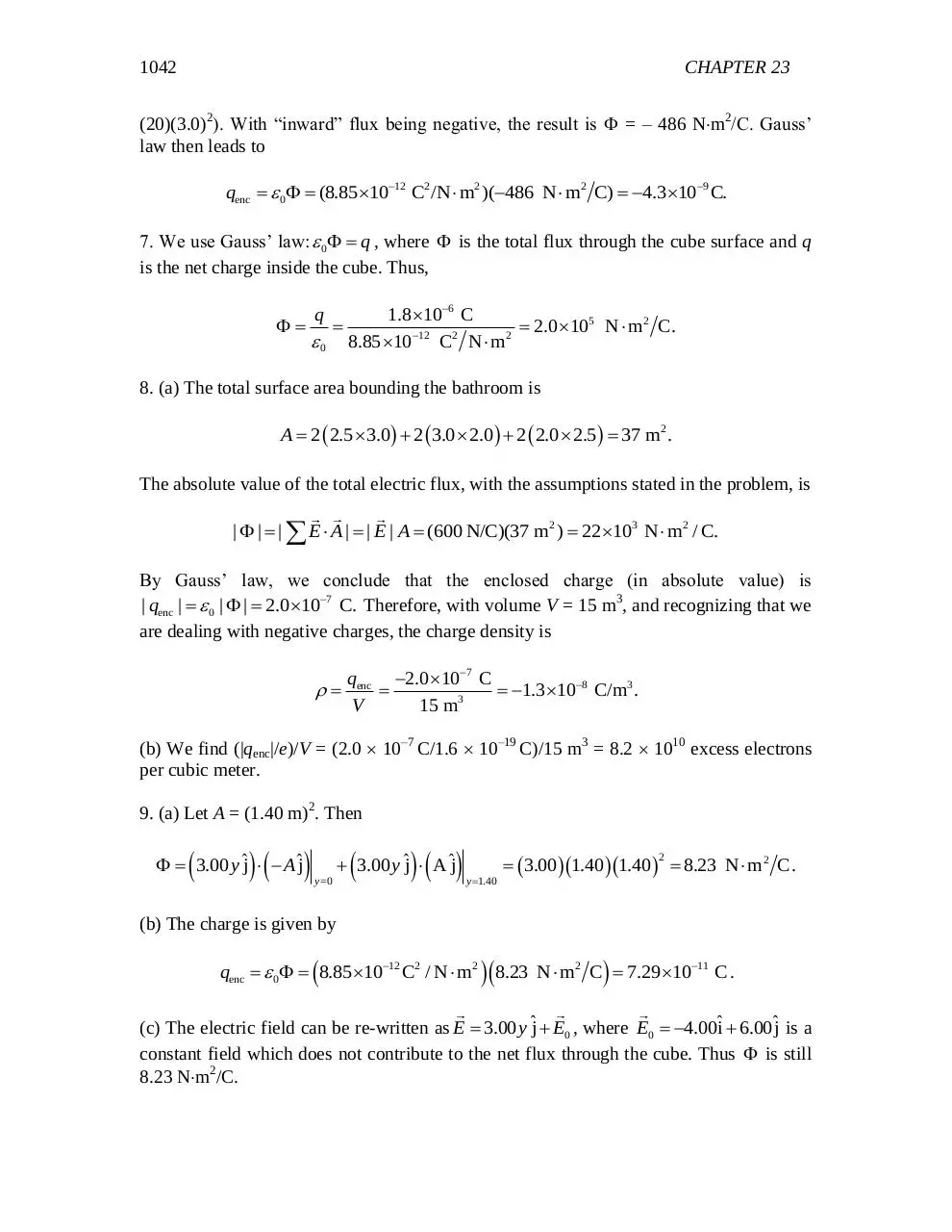
9. (a) Let A = (1.40 m)2. Then



 

  3.00 y ˆj   A ˆj



 

 3.00 y ˆj  A ˆj
y =0

  3.00 1.40 1.40   8.23 N  m2 C.
2

y 1.40

(b) The charge is given by







qenc   0  8.85 1012 C2 / N  m2 8.23 N  m2 C  7.29 1011 C .

(c) The electric field can be re-written as E  3.00 y ˆj  E0 , where E0  4.00iˆ  6.00jˆ is a
constant field which does not contribute to the net flux through the cube. Thus  is still
8.23 Nm2/C.

1043
(d) The charge is again given by







qenc   0  8.85 1012 C2 / N  m2 8.23 N  m2 C  7.29 1011 C .

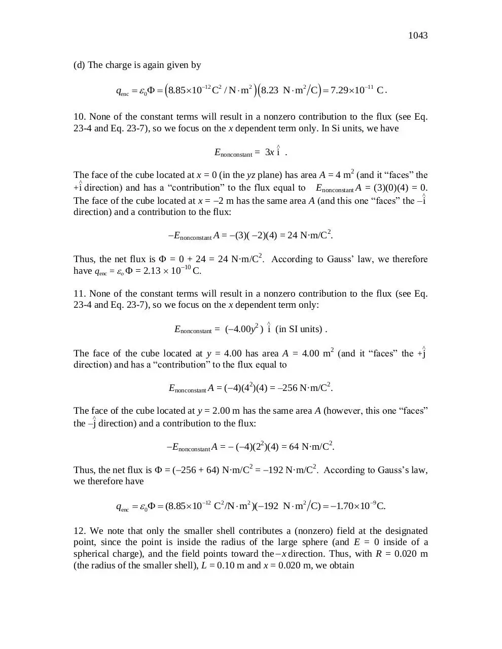
10. None of the constant terms will result in a nonzero contribution to the flux (see Eq.
23-4 and Eq. 23-7), so we focus on the x dependent term only. In Si units, we have
^

Enonconstant = 3x i .
The face of the cube located at x = 0 (in the yz plane) has area A = 4 m2 (and it “faces” the
^
+i direction) and has a “contribution” to the flux equal to Enonconstant A = (3)(0)(4) = 0.
^
The face of the cube located at x = 2 m has the same area A (and this one “faces” the –i
direction) and a contribution to the flux:
Enonconstant A = (3)(2)(4) = 24 N·m/C2.
Thus, the net flux is  = 0 + 24 = 24 N·m/C2. According to Gauss’ law, we therefore
have qenc =  = 2.13  1010 C.
11. None of the constant terms will result in a nonzero contribution to the flux (see Eq.
23-4 and Eq. 23-7), so we focus on the x dependent term only:
^

Enonconstant = (4.00y2 ) i (in SI units) .
^

The face of the cube located at y = 4.00 has area A = 4.00 m2 (and it “faces” the +j
direction) and has a “contribution” to the flux equal to
Enonconstant A = (4)(42)(4) = –256 N·m/C2.

The face of the cube located at y = 2.00 m has the same area A (however, this one “faces”
^
the –j direction) and a contribution to the flux:
Enonconstant A =  (4)(22)(4) =  N·m/C2.
Thus, the net flux is  = (256 + 64) N·m/C2 = 192 N·m/C2. According to Gauss’s law,
we therefore have

qenc   0  (8.85 1012 C2 /N  m2 )(192 N  m2 C)  1.70 109 C.
12. We note that only the smaller shell contributes a (nonzero) field at the designated
point, since the point is inside the radius of the large sphere (and E = 0 inside of a
spherical charge), and the field points toward the  x direction. Thus, with R = 0.020 m
(the radius of the smaller shell), L = 0.10 m and x = 0.020 m, we obtain

1044

CHAPTER 23
E  E (ˆj)  


q
4 0 r

ˆj  
2

4 R 2 2 ˆ
R 2 2 ˆ
j 
j
4 0 ( L  x) 2
 0 ( L  x) 2

(0.020 m) 2 (4.0 106 C/m 2 )
ˆj   2.8 104 N/C  ˆj .
12
2
2
2
(8.85 10 C /N  m )(0.10 m  0.020 m)

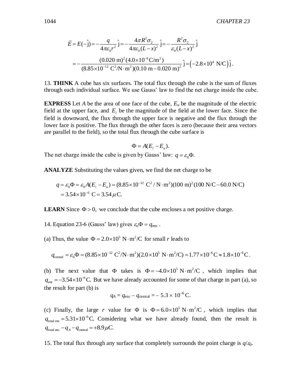
13. THINK A cube has six surfaces. The total flux through the cube is the sum of fluxes
through each individual surface. We use Gauss’ law to find the net charge inside the cube.
EXPRESS Let A be the area of one face of the cube, Eu be the magnitude of the electric
field at the upper face, and El be the magnitude of the field at the lower face. Since the
field is downward, the flux through the upper face is negative and the flux through the
lower face is positive. The flux through the other faces is zero (because their area vectors
are parallel to the field), so the total flux through the cube surface is

  A( E  Eu ).
The net charge inside the cube is given by Gauss’ law: q   0.
ANALYZE Substituting the values given, we find the net charge to be

q   0   0 A( E  Eu )  (8.85 1012 C2 / N  m 2 )(100 m) 2 (100 N/C  60.0 N/C)
 3.54 106 C  3.54  C.
LEARN Since   0, we conclude that the cube encloses a net positive charge.
14. Equation 23-6 (Gauss’ law) gives qenc .
(a) Thus, the value   2.0 105 N  m2 /C for small r leads to

qcentral   0  (8.85 1012 C2 /N  m2 )(2.0 105 N  m2 /C)  1.77 106 C  1.8 106 C 
(b) The next value that  takes is   4.0 105 N  m2 /C , which implies that
qenc  3.54 106 C. But we have already accounted for some of that charge in part (a), so
the result for part (b) is
qA = qenc – qcentral = – 5.3  106 C.
(c) Finally, the large r value for  is   6.0 105 N  m2 /C , which implies that
qtotal enc  5.31106 C. Considering what we have already found, then the result is
qtotal enc  qA  qcentral  8.9C.
15. The total flux through any surface that completely surrounds the point charge is q/0.

1045
(a) If we stack identical cubes side by side and directly on top of each other, we will find
that eight cubes meet at any corner. Thus, one-eighth of the field lines emanating from
the point charge pass through a cube with a corner at the charge, and the total flux
through the surface of such a cube is q/80. Now the field lines are radial, so at each of
the three cube faces that meet at the charge, the lines are parallel to the face and the flux
through the face is zero.
(b) The fluxes through each of the other three faces are the same, so the flux through each
of them is one-third of the total. That is, the flux through each of these faces is (1/3)(q/80)
= q/240. Thus, the multiple is 1/24 = 0.0417.
16. The total electric flux through the cube is    E  dA . The net flux through the two
faces parallel to the yz plane is

 yz    Ex ( x  x2 )  Ex ( x  x1 )  dydz  
 6

y2 1
y1  0

dy 

z2  3

z1 1

y2 1
y1  0

dy 

z2  3

z1 1

dz 10  2(4) 10  2(1) 

dz  6(1)(2)  12.

Similarly, the net flux through the two faces parallel to the xz plane is

 xz    Ey ( y  y2 )  E y ( y  y1 )  dxdz  

x2  4

x1 1

dy 

z2 3

z1 1

dz[3  (3)]  0 ,

and the net flux through the two faces parallel to the xy plane is
 xy    Ez ( z  z2 )  Ez ( z  z1 ) dxdy  

x2  4

x1 1

dx 

y2 1

y1 0

dy  3b  b   2b(3)(1)  6b.

Applying Gauss’ law, we obtain
qenc   0   0 ( xy   xz   yz )   0 (6.00b  0 12.0)  24.0 0

which implies that b = 2.00 N/C  m .
17. THINK The system has spherical symmetry, so our Gaussian surface is a sphere of
radius R with a surface area A  4 R2 .
EXPRESS The charge on the surface of the sphere is the product of the surface charge
density  and the surface area of the sphere: q   A   (4 R2 ). We calculate the total
electric flux leaving the surface of the sphere using Gauss’ law: q   0.
ANALYZE (a) With R  (1.20 m) / 2  0.60 m and   8.1106 C/m2 , the charge on
the surface is

1046

CHAPTER 23
q  4R2  4  0.60 m  (8.1106 C/m2 )  3.7 105 C.
2

(b) We choose a Gaussian surface in the form of a sphere, concentric with the conducting
sphere and with a slightly larger radius. By Gauss’s law, the flux is


q

0

3.66 105 C
 4.1106 N  m2 / C .
8.85 1012 C2 / N  m 2



LEARN Since there is no charge inside the conducting sphere, the total electric flux
through the surface of the sphere only depends on the charge residing on the surface of
the sphere.
18. Using Eq. 23-11, the surface charge density is

  E 0   2.3 105 N C8.85 1012C2 / N  m2   2.0 106 C/m2 .
19. (a) The area of a sphere may be written 4R2= D2. Thus,



q
2.4 106 C

 4.5 107 C/m2 .
2
2
D
 1.3 m 

(b) Equation 23-11 gives
E


4.5 107 C/m2

 5.1104 N/C.
12
2
2
 0 8.85 10 C / N  m

20. Equation 23-6 (Gauss’ law) gives qenc.
(a) The value   9.0 105 N  m2 /C for small r leads to qcentral = – 7.97  106 C or
roughly – 8.0 C.
(b) The next (nonzero) value that  takes is   4.0 105 N  m2 /C , which implies
qenc  3.54 106 C. But we have already accounted for some of that charge in part (a), so
the result is
qA = qenc – qcentral = 11.5  106 C  12  C .
(c) Finally, the large r value for  is   2.0 105 N  m2 /C, which implies
qtotal enc  1.77 106 C. Considering what we have already found, then the result is

qtotal enc – qA  qcentral = –5.3 C.
21. (a) Consider a Gaussian surface that is completely within the conductor and surrounds
the cavity. Since the electric field is zero everywhere on the surface, the net charge it

1047
encloses is zero. The net charge is the sum of the charge q in the cavity and the charge qw
on the cavity wall, so q + qw = 0 and qw = –q = –3.0  10–6C.
(b) The net charge Q of the conductor is the sum of the charge on the cavity wall and the
charge qs on the outer surface of the conductor, so Q = qw + qs and



 



qs  Q  q  10 106 C  3.0 106 C  1.3 105 C.

22. We combine Newton’s second law (F = ma) with the definition of electric field
( F  qE ) and with Eq. 23-12 (for the field due to a line of charge). In terms of
magnitudes, we have (if r = 0.080 m and   6.0 106 C/m )
ma = eE =

e
2o r



a=

e
= 2.1  1017 m/s2 .
2o r m

23. (a) The side surface area A for the drum of diameter D and length h is given by
A   Dh . Thus,
q   A   Dh   0 EDh







  8.85 1012 C2 /N  m 2 2.3 105 N/C  0.12 m  0.42 m 
 3.2 10

7

C.

(b) The new charge is
 A 
  Dh 
7
q  q    q 
  3.2 10 C
A

Dh
 





 8.0 cm  28 cm  

  12 cm  42 cm    1.4 10




7

C.

24. We imagine a cylindrical Gaussian surface A of radius r and unit length concentric
q
with the metal tube. Then by symmetry  E  dA  2rE  enc .

0

A

(a) For r < R, qenc = 0, so E = 0.
(b) For r > R, qenc = , so E (r )   / 2 r 0 . With   2.00 108 C/m and r = 2.00R =
0.0600 m, we obtain

 2.0 10 C/m 
E
2  0.0600 m  8.85 10 C
8

12

2

/ Nm

2



 5.99 103 N/C.

(c) The plot of E vs. r is shown to the right. Here, the
maximum value is

1048

CHAPTER 23

Emax





2.0 108 C/m



 1.2 104 N/C.
12
2
2
2 r 0 2  0.030 m  8.85 10 C / N  m





25. THINK Our system is an infinitely long line of charge. Since the system possesses
cylindrical symmetry, we may apply Gauss’ law and take the Gaussian surface to be in
the form of a closed cylinder.
EXPRESS We imagine a cylindrical Gaussian surface A of radius r and length h
concentric with the metal tube. Then by symmetry,



A

E  dA  2 rhE 

q

0

,

where q is the amount of charge enclosed by the Gaussian cylinder. Thus, the magnitude
of the electric field produced by a uniformly charged infinite line is
E

q/h


2 0 r 2 0 r

where  is the linear charge density and r is the distance from the line to the point where
the field is measured.
ANALYZE Substituting the values given, we have

  2 0 Er  2 8.85 1012 C2 / N  m2  4.5 104 N/C   2.0 m 
 5.0 106 C/m.
LEARN Since   0, the direction of E is radially outward from the line of charge.
Note that the field varies with r as E 1/ r, in contrast to the 1/ r 2 dependence due to a
point charge.
26. As we approach r = 3.5 cm from the inside, we have
Einternal 

2
4 0 r

 1000 N/C .

And as we approach r = 3.5 cm from the outside, we have
Eexternal 

2
4 0 r



2 
 3000 N/C .
4 0 r