Diff EQ (PDF)

Spring 2017

MA 262
Study Guide - Exam # 1 (Part A)
1 Solutions to Special Types of 1st Order Equations:
I Separable Equation (SEP):
Solution Method :

p(y)

dy
= q(x), or equivalently, p(y) dy = q(x) dx
dx

Solution y = y(x) is given implicitly by
∫
∫
p(y) dy = q(x) dx

B There may be additional constant solutions y ≡ K which arise if you divide by expressions involving y.
You must check to see if there are additional solutions.

II First Order Linear Equation (FOL):

Solution Method :

1
y=
I(x)

[∫

dy
+ p(x) y = q(x) (Standard Form)
dx
]

∫

I(x) q(x) dx + C , for an integrating factor I(x) = e

p(x) dx

.

B The FOL equation must be in Standard Form.
dy
= f (x, y) , where f (tx, ty) = f (x, y), t > 0
dx
dy
dV
y
Solution Method : Let
V (x) =
. Hence y = xV (x) and so
=x
+V.
x
dx
dx
This change of variables transforms the original Homogeneous equation into a Separable equation iny
volving V . Solve the resulting Separable equation and then remember V = .
x
There may be extra solutions.
III Homogeneous Equation (HOM):

B

IV Bernoulli Equation (BER):

dy
+ p(x)y = q(x)y n , (n ̸= 0, 1)
dx

Solution Method : Divide the equation by y n to get:
Let

u = y 1−n

and so

y −n

dy
dx

+ p(x)y 1−n = q(x) (∗)

du
dy
dy
1
du
= (1 − n)y −n
. Thus, y −n
=
.
dx
dx
dx
(1 − n) dx

This change of variables transforms the original Bernoulli equation into a First Order Linear equation
involving u. Substitute these into (∗) and solve the resulting First Order Linear Equation for u and then
remember u = y 1−n .

V Exact Equation (EXE):

M (x, y) dx + N (x, y) dy = 0, where

Solution Method : Solution y = y(x) given implicitly by an equation
function ϕ(x, y) is determined by either of these methods:
(a) Book method:

∂ϕ


= M (x, y)


∂x















∂ϕ


= N (x, y)

∂y

Ix
=⇒

∂M
∂N
=
∂y
∂x

ϕ(x, y) = C

where the

∫
ϕ(x, y) =

M (x, y) dx + h(y)

w
w
w Dy

∂ϕ
∂
=
∂y
∂y

(∫

)

M (x, y) dx + h′ (y) (#)
∫
==
> Find the function h(y) in equation (#) and hence ϕ(x, y) = M (x, y) dx + h(y).
(b) Student method:

∂ϕ


= M (x, y)

 ∂x

==

Ix
=⇒

∫
ϕ(x, y) =

M (x, y) dx + h(y) (∗)

∫


∂ϕ
I
y


= N (x, y)
ϕ(x, y) = N (x, y) dy + g(x) (∗∗)
∂y
=⇒
==
> Compare the two forms (*) and (**) and determine suitable ϕ(x, y).
The function

ϕ(x, y) is called a potential function for the differential equation.

VI Other 1st Order Equations: If possible, use suitable change of variables or other techniques to
convert original differential equation to one of the previous types I - V .

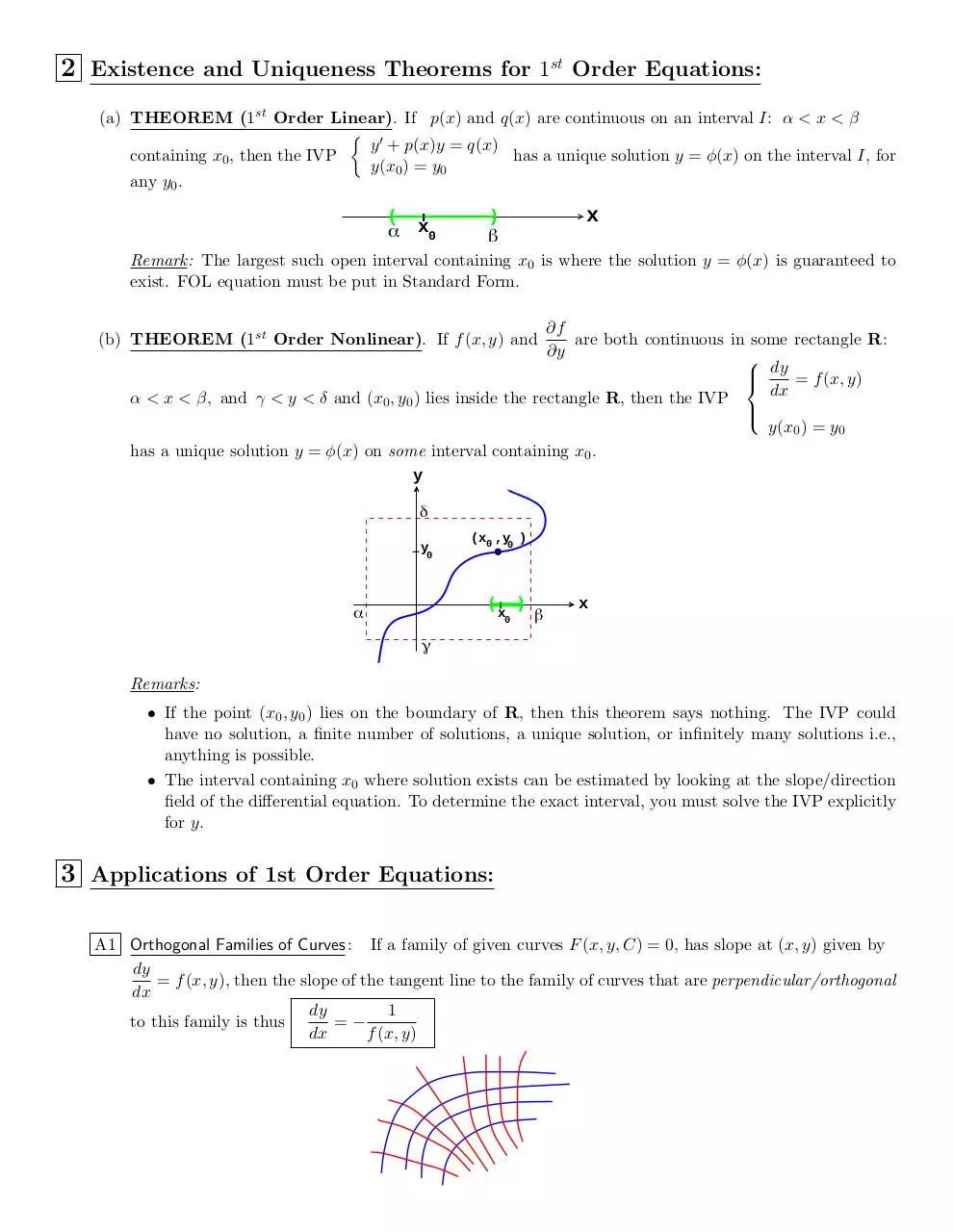
2 Existence and Uniqueness Theorems for 1st Order Equations:
(a) THEOREM (1st Order Linear). If p(x) and q(x) are continuous on an interval I: α < x < β
{ ′
y + p(x)y = q(x)
containing x0 , then the IVP
has a unique solution y = ϕ(x) on the interval I, for
y(x0 ) = y0
any y0 .

(
α x0

x

)
β

Remark: The largest such open interval containing x0 is where the solution y = ϕ(x) is guaranteed to
exist. FOL equation must be put in Standard Form.
∂f
are both continuous in some rectangle R:
∂y

dy


= f (x, y)
dx
α < x < β, and γ < y < δ and (x0 , y0 ) lies inside the rectangle R, then the IVP


y(x0 ) = y0
has a unique solution y = ϕ(x) on some interval containing x0 .
y

(b) THEOREM (1st Order Nonlinear). If f (x, y) and

δ
y0

(x0 ,y0 )

(x )

α

0

β

x

γ

Remarks:
• If the point (x0 , y0 ) lies on the boundary of R, then this theorem says nothing. The IVP could
have no solution, a finite number of solutions, a unique solution, or infinitely many solutions i.e.,
anything is possible.
• The interval containing x0 where solution exists can be estimated by looking at the slope/direction
field of the differential equation. To determine the exact interval, you must solve the IVP explicitly
for y.

3 Applications of 1st Order Equations:
A1 Orthogonal Families of Curves : If a family of given curves F (x, y, C) = 0, has slope at (x, y) given by
dy
= f (x, y), then the slope of the tangent line to the family of curves that are perpendicular/orthogonal
dx
dy
1
to this family is thus
=−
dx
f (x, y)

A2 Malthusian Population Growth :

P (t) = population at time t
dP
= kP
dt

The solution is P (t) = P0 ekt .
1
ln 2.
k

Time to double population, doubling time, tD =
A3 Logistic Population Growth :

The solution is P (t) =

P (t) = population at time t
(
)
dP
P
= rP 1−
where r, C > 0
dt
C

P0 C
.
P0 + (C − P0 ) e−rt

C is called the Carrying Capacity of the population.
A4 Mixing Problems :

ri
ci

A(t) = amount of substance in tank at time t
V (t) = volume of solution in tank at time t
dA
= ri ci − ro co ,
dt

A5 Newton’s Law of Cooling :

where

c0 =

A(t)
V (t)
ro
co

T (t) = temperature at time t
Tm = temperature of surrounding medium
dT
= −k (T − Tm ), k > 0
dt

A6 RLC Circuits :
Kirchoff ’s 2nd

dq
= current
dt
Law : Voltage drop around closed circuit is zero. Hence
q(t) = charge; i(t) =

L

di
q
+Ri+
= E(t)
dt
C

.

.
.

E(t)

.

L
EMF

C
.

R
Equivalently, L

d2 q
q
dq
+R
+
= E(t).
2
dt
dt
C

.

.
.

.

dv
d2 y
= m 2 . Near the surface of the Earth, the force
dt
dt
due to gravity is the weight of the object Fg = mg. For the two cases below (no air resistance) we have:

A7 Falling/Rising Objects : Newton’s 2nd Law: F = m

(a)
.

m

d2 y
= mg
dt2

and

(b)

m

.

.

.

.

d2 y
= −mg
dt2

.
.

(a) Falling Body
+ y direction

.

(b) Rising Body

m

m

Fg = mg

Fg = mg

+ y direction
.

.

.

.

.
.
.

.
.

nd

4 Special Types of 2 Order Equations :

(
)
dy
d2 y
= F x, y,
dx2
dx

(
)
d2 y
dy
i No Dependent Variable (Missing y) :
= F x,
(∗)
dx2
dx
d2 y
dy
dv
= v(x) and hence
=
to convert the 2nd order equation (∗) to a 1st
2
dx
dx
dx
dy
order equation in v(x) and solve it for v(x). Then since
= v(x), solve this 1st order equation for y.
dx
(
)
d2 y
dy
ii No Independent Variable (Missing x) :
= F y,
(∗∗)
dx2
dx
Use the substitution

Use the substitution

dy
= v(y) and, by the Chain Rule,
dx

dv
d2 y
=v
2
dx
dy

to convert the 2nd order

dy
equation (∗∗) to a 1st order equation in v(y) and solve it for v(y). Then since
= v(y), solve this 1st
dx
order equation for y.
dy
= f (x, y) has slope f (x, y)
dx
at the point (x, y). The slope field (or direction field) of the d.e. indicates the slope of solutions at various
points (x, y):

5 Slope Fields (Direction Fields): A solution y = ϕ(x) to the d.e.

Slope field for

dy
= f (x, y)
dx

Slope field and solutions to

dy
= f (x, y)
dx

• To sketch slope fields, usually consider where the slopes are constant k. Thus on the curves given by
dy
= f (x, y) all have constant slope k along these curves. Such curves are
f (x, y) = k, the solutions to
dx
called isoclines.
• If the d.e. has a constant solution y ≡ L, it is called an equilibrium solution to the d.e.
d2 y
.
dx2
• The direction field may be used to give qualitative information about the behavior of solutions as x → ∞
(or x → −∞, or x → 0, etc). Slope fields may also be used to estimate the interval where a solution
through a point (x0 , y0 ) is defined.
• The concavity of solutions are determined by the sign of