Report performance analysis AC (PDF)

Performance analysis of an air conditioner in domestic setting using
CFD simulation
In today’s world air conditioning is almost used everywhere for the human comfort. Thus,
analyzing the performance of air conditioning and temperature distribution of the air conditioned
is essential. This model work focused on numerical study of temperature distribution of an air
conditioned room and performance of a 1.5 ton rating air conditioner (AC) using CFD simulation.

Figure 1. Model room with an air conditioner
The model room with an air conditioner is shown in the above figure. The closed room with a
dimension of 12m x 12m x 2.5m and air conditioner inlet opening length of 1m. Two slits in the
AC are used as an Inlet. The numerical domain (mesh) is created using Hex-dominant parametric
method. The final mesh consist of 2.8 million cells and all the mesh quality parameters are passed.
The final meshed model is shown in the figure below.

Figure 2. Finalized mesh of the model (room with an AC)
The model is finely meshed using volume, surface, layer and edge refinement options. To get an
accurate and reliable results from the mesh then the 𝑦 value should be in the range of 30 to
300 (log law region). Because, if the 𝑦 value is higher than the range, then wall function of
turbulence model may incorrectly calculate the flow properties. The wall function is not necessary,

if the 𝑦 value is less than 5 (viscous sub layer) but it need more number of cells near the
boundary layer.
The custom type boundary condition is used in this simulations. The air conditioner is an inlet
and set to fixed temperature of 290K, 291K & 293K with fixed velocity (zero) and fixed flux
pressure. The room wall has the heat transfer coefficient as 0.5 𝑊⁄𝑚 𝐾 with ambient temperature
is assumed as 313 K, fixed velocity (zero) and fixed flux pressure. The other AC parts (surface)
are set to temperature gradient to zero with fixed velocity (zero) and fixed flux pressure. The
steady state convective heat transfer solver with K-omega SST turbulence is selected for this
numerical simulation.
One of the deficiencies of the k-ε model is its inability to handle low turbulent Reynolds number
computations as well as the requirement of highly refined near-wall grid resolution in an attempt
to model low turbulent Reynolds number flows. This approach often leads to numerical instability.
Some of these difficulties may be avoided by using the k-omega model, making it more
appropriate than the k-ε model for flows requiring high near-wall resolution (for example, high
wall heat transfer, and transition). Thus SST K-omega model is selected over the k-ε model. SST
K-omega model is combination of a k-omega model (in the inner boundary layer) and k-ε model
(in the outer region of and outside of the boundary layer). The SST k-omega model is
recommended for accurate boundary layer simulations.
The simulations were carried out for three different AC temperature 290 K, 291 K and 293 K with
other boundary conditions as same. The simulation was carried out for 3000 iterations with 32
core and it ran for approximately 5 hours. The figure below shows the converged results of an
area-averaged temperature on each wall of the room. The simulation is started to converge from
1500th iterations.

Figure 3. Convergence behavior for the temperature (area averaged) of the room walls

Performance analysis of an air conditioner:
Coefficient of performance (COP):
The COP is a measure of the amount of power input to a system compared to the amount of
power output by that system.
𝐶𝑂𝑃 =

𝑃𝑜𝑤𝑒𝑟 𝑜𝑢𝑡𝑝𝑢𝑡
𝑃𝑜𝑤𝑒𝑟 𝑖𝑛𝑝𝑢𝑡

An air conditioning system uses power to move heat from one place to another place. When
cooling, the air conditioning system is moving heat from the room to the outside environment. The
maximum COP for an air conditioning system is expressed by Carnot’s theorem, reduced to the
following equation,
𝐶𝑂𝑃

=

𝑇
𝑇 −𝑇

Where, 𝑇 is temperature of the room and 𝑇 is ambient temperature. The 𝑇 is calculated by
taking average of the room temperature (using paraview).
Air conditioner
temperature (K)
290
291
293

𝑇 (average)
(K)
297.38
297.83
303.74

𝑇 (Fixed)
(K)
313
313
313

𝐶𝑂𝑃
19.05
19.63
32.8

The computed COP is very high because it is a theoretical maximum value of air conditioner,
Typical COP of air conditioner values would be in the range 2 to 4 or approximately one tenth of
a theoretical maximum value. Therefore actual COP value of air conditioner is shown below table.
Air conditioner
temperature (K)
290
291
293

𝑇 (average)
(K)
297.38
297.83
303.74

𝑇 (Fixed)
(K)
313
313
313

𝐶𝑂𝑃
19.05
19.63
32.8

𝐶𝑂𝑃
(approximated)
1.90
1.96
3.28

Power Consumption:
1 TR is defined as the heat removal rate so as to freeze 1 ton (1000 kg) of water at 0°C into ice
at 0°C in twenty-four hours. In actual practice, one TR is equivalent to 210 kJ/min or 3.5 kJ/s. In
this simulation, we assumed our AC has rating of 1.5 ton. We know that,
𝐶𝑂𝑃 =

𝑃𝑜𝑤𝑒𝑟 𝑜𝑢𝑡𝑝𝑢𝑡
3.5 ∗ 𝐶𝑎𝑝𝑎𝑐𝑖𝑡𝑦
=
𝑃𝑜𝑤𝑒𝑟 𝑖𝑛𝑝𝑢𝑡
𝑃𝑜𝑤𝑒𝑟 𝑐𝑜𝑛𝑠𝑢𝑚𝑒𝑑 𝑏𝑦 𝑡ℎ𝑒 𝑐𝑜𝑚𝑝𝑟𝑒𝑠𝑠𝑜𝑟

𝑃𝑜𝑤𝑒𝑟 𝑐𝑜𝑛𝑠𝑢𝑚𝑒𝑑 𝑏𝑦 𝑡ℎ𝑒 𝑐𝑜𝑚𝑝𝑟𝑒𝑠𝑠𝑜𝑟 =

3.5 ∗ 1.5
𝐶𝑂𝑃

Air conditioner
temperature (kelvin)
290
291
293

𝐶𝑂𝑃
(approximated)
1.90
1.96
3.28

Power Consumption
(Watt)
2763.15
2674.47
1600.60

From the above table we can deduce that more power consumption is required for low room temperature
because more electrical input needed to remove the heat from the room to outside.

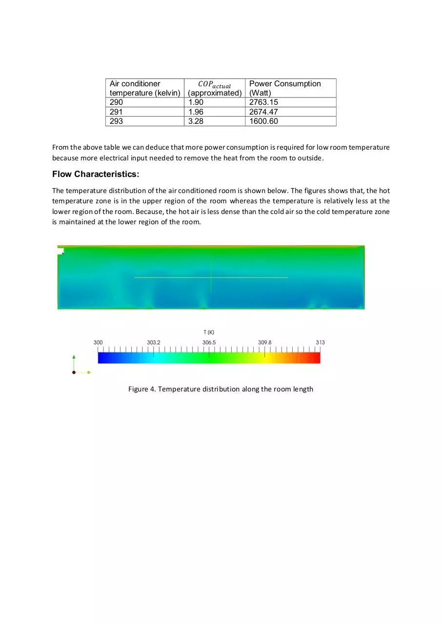
Flow Characteristics:
The temperature distribution of the air conditioned room is shown below. The figures shows that, the hot
temperature zone is in the upper region of the room whereas the temperature is relatively less at the
lower region of the room. Because, the hot air is less dense than the cold air so the cold temperature zone
is maintained at the lower region of the room.

Figure 4. Temperature distribution along the room length

Figure 5. Temperature distribution inside the room.

Figure 6. Cold Temperature zone in the room. (Average temperature is 303.8K)

Figure 7. Velocity distribution inside the room.