SuppHelmholtzDecomposition (PDF)

Helmholtz Decomposition of Vector Fields
Dr. Christopher S. Baird
University of Massachusetts Lowell

1. Introduction
The Helmholtz Decomposition Theorem, or the fundamental theorem of vector calculus, states that any
well-behaved vector field can be decomposed into the sum of a longitudinal (diverging, non-curling,
irrotational) vector field and a transverse (solenoidal, curling, rotational, non-diverging) vector field.
Here, the terms “longitudinal” and “transverse” refer to the nature of the operators and not the vector
fields. A purely “transverse” vector field does not necessarily have all of its vectors perpendicular to
some reference vector. In one sense, the divergence and curl operators can be thought of as orthogonal
operators as their product is zero and they extract independent parts of a general vector field. This is
demonstrated in the mathematical identities:
∇×∇ Φ=0 and ∇⋅(∇×A)=0
There is also a third part to a general vector field. Even if the curl and divergence of a vector field is
zero, the vector field can still be non-zero and non-trivial. This third part is known as the Laplacian part
or the relaxed part and is contained in the other parts.
2. Proof
Start with a general vector field F(x) where x is the three-dimensional observation point vector.
Expand F into an integral including a Dirac delta:
F( x)=∫V F(x ')δ (x−x ') d x '

Here, we leave the integration volume V arbitrary for the sake of generality; it does not have to be all
space, but it does have to include the point x. Now use the identity:
δ( x−x ')=−

(

)

1
1
∇2
4π
∣x−x '∣

to find:
F( x)=−

F( x ')
1
2
∇ ∫V
d x'
∣x−x '∣
4π

Now use the identity ∇ 2 A=∇ (∇⋅A)−∇ ×( ∇ ×A) to find:
F( x)=−

(

)

(

F( x ')
F( x ')
1
1
∇ ∇⋅∫V
d x' +
∇ × ∇ ×∫V
d x'
∣x−x '∣
∣x−x '∣
4π
4π

)

Identify the first term as the longitudinal part Fl and the second term as the transverse part Ft:

F=Fl +Ft where Fl =−

(

F(x ')
1
∇ ∇⋅∫V
d x'
∣
4π
x−x '∣

)

and Ft =

(

F( x ')
1
∇ × ∇×∫V
d x'
∣
4π
x−x '∣

)

Taking the curl of Fl shows that it is indeed non-curling (longitudinal), and taking the divergence of Ft
shows that it is indeed non-diverging (transverse) as follows:
∇×Fl =−

(

F( x ')
1
∇ ×∇ ∇⋅∫V
d x'
∣x−x '∣
4π

)

∇×Fl =0 because the curl of the gradient is always zero
∇⋅Ft=

(

F(x ')
1
∇⋅∇ × ∇ ×∫V
d x'
∣x−x '∣
4π

)

∇⋅Ft=0 because the divergence of the curl is always zero

This means that the one term is purely solenoidal and the other is purely diverging and their sum gives
a general vector field. This is the Helmholtz Decomposition Theorem. Summarized mathematically, we
have:
F=Fl +Ft where ∇⋅F=∇⋅Fl and ∇×F=∇ ×Ft
3. Field Sources
Let us investigate further. The field that results when we take the divergence of F we will call the
source of F's divergence. It is apparently a scalar field ψ. Similarly, the field that results when we take
the curl of F we will call the source of F's curling nature. It is a vector field U.
ψ=∇⋅F
U=∇×F

Both ψ and U are source fields; they are not the vector field components of F but are related to them.
According to the Helmholtz Decomposition Theorem, this immediately tells us:
ψ=∇⋅Fl
U=∇×Ft

Let us go back to the expansion of F and see if we can get them to appear.
F( x)=−

(

)

(

F( x ')
F( x ')
1
1
∇ ∇⋅∫V
d x' +
∇ × ∇ ×∫V
d x'
∣
∣
∣
4π
x−x '
4π
x−x '∣

)

Use ∇⋅(Φ A)=A⋅∇ Φ+Φ ∇⋅A on the first term realizing that F is a function of primed variables only
so the divergence of F with respect to unprimed variables is zero. Similarly, use
∇×(Φ A)=Φ ∇×A+(∇ Φ)×A on the second term realizing that the curl of F with respect to

unprimed variables is zero for the same reason. After applying both of these expansions, we find:
F( x)=−

1
∇
4π

(∫

V

F( x ')⋅∇

(∣ ∣)

(

(∣ ∣) )

(∫

1
1
d x' −
∇×
x−x '
4π

V

F(x ')×∇

(∣ ∣) )
1
d x'
x−x '

)

1
1
=−∇ '
where the prime on the gradient operator denotes differentiation with
x−x '
∣x−x '∣
respect to the primed variables.
Use ∇

F(x)=

1
∇
4π

(∫

V

F(x ')⋅∇ '

(∣ ∣) )

(∫

1
1
d x' +
∇×
x−x '
4π

V

F( x ')×∇ '

(∣ ∣) )
1
d x'
x−x '

Use ∇⋅(Φ A)=A⋅∇ Φ+Φ ∇⋅A and ∇×(Φ A)=Φ ∇×A+( ∇ Φ)×A again but now with respect to
primed variables such that:
F(x ')⋅∇ '

(∣ ∣) (∣ ∣)

F (x ')
∇ '⋅F(x ')
1
=∇ '⋅
−
∣x−x '∣
x−x '
x−x '

F(x ')×∇ '

(

(∣ ∣)

and

)

F(x ')
∇ '×F(x ')
1
=−∇ '×
+
∣x−x '∣
∣x−x '∣
x−x '

Using these two expansions, the total expression for F becomes:
F(x)=
+

1
∇
4π

(∫ ( ) ∫
(∫ ( )
V

∇ '⋅

1
∇× [−
4π

V

F( x ')
d x '−
∣x−x '∣

∇ '×

V

∇ '⋅F(x ')
d x'
∣x−x '∣

)

)

F (x ')
∇ '×F( x ')
d x '+∫V
d x ']
∣x−x '∣
∣x−x '∣

We can use the divergence theorem on the first term to turn it into a surface integral over the surface S
bounding volume V. If we let V be all space, then S is the surface at infinity. If F is well-behaved, it will
die off to zero at infinity and this surface integral vanishes. Similarly, we can use a version of Stokes
theorem on the third term to reduce it down to a surface integral over S. This term will also go away if
the volume is all space and F is well-behaved. With these two terms gone, we have:
F(x)=−

Now use ∇

F( x)=

(

)

(

)

1
1
1
1
d x '−
d x'
( ∇ '⋅F( x ') ) ∇
( ∇ '×F(x ') )×∇
∫
∫
4π
∣x−x '∣
4π
∣x−x '∣

(∣ ∣)

1
x−x '
=−
to find:
x−x '
∣x−x '∣3

(x−x ')
(x−x ')
1
1
( ∇ '⋅F(x ') )
d x '+
( ∇ '×F(x '))×
d x'
∫
∫
3
4π
4π
∣x−x '∣
∣x−x '∣3

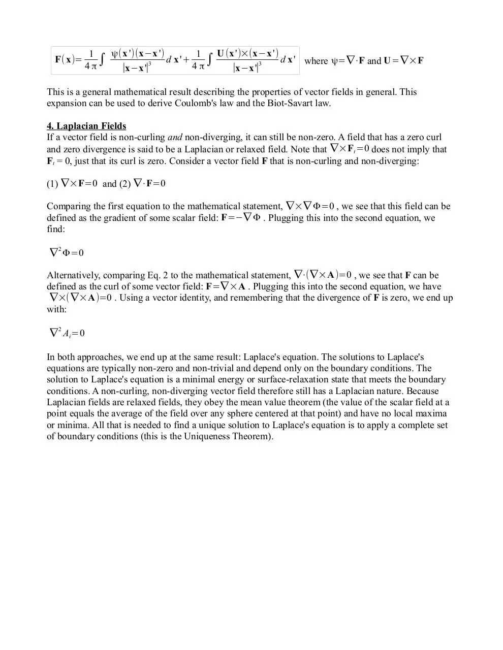
Now identity the sources, ψ=∇⋅F and U=∇×F inside the integrals:

F( x)=

ψ( x ')(x−x ')
U (x ')×(x−x ')
1
1
d x '+
d x ' where ψ=∇⋅F and U=∇×F
∫
∫
3
4π
4π
∣x−x '∣
∣x−x '∣3

This is a general mathematical result describing the properties of vector fields in general. This
expansion can be used to derive Coulomb's law and the Biot-Savart law.
4. Laplacian Fields
If a vector field is non-curling and non-diverging, it can still be non-zero. A field that has a zero curl
and zero divergence is said to be a Laplacian or relaxed field. Note that ∇×Ft =0 does not imply that
Ft = 0, just that its curl is zero. Consider a vector field F that is non-curling and non-diverging:
(1) ∇×F=0 and (2) ∇⋅F=0
Comparing the first equation to the mathematical statement, ∇×∇ Φ=0 , we see that this field can be
defined as the gradient of some scalar field: F=−∇ Φ . Plugging this into the second equation, we
find:
2

∇ Φ=0

Alternatively, comparing Eq. 2 to the mathematical statement, ∇⋅(∇×A)=0 , we see that F can be
defined as the curl of some vector field: F=∇ ×A . Plugging this into the second equation, we have
∇×(∇×A)=0 . Using a vector identity, and remembering that the divergence of F is zero, we end up
with:
∇ 2 Ai=0
In both approaches, we end up at the same result: Laplace's equation. The solutions to Laplace's
equations are typically non-zero and non-trivial and depend only on the boundary conditions. The
solution to Laplace's equation is a minimal energy or surface-relaxation state that meets the boundary
conditions. A non-curling, non-diverging vector field therefore still has a Laplacian nature. Because
Laplacian fields are relaxed fields, they obey the mean value theorem (the value of the scalar field at a
point equals the average of the field over any sphere centered at that point) and have no local maxima
or minima. All that is needed to find a unique solution to Laplace's equation is to apply a complete set
of boundary conditions (this is the Uniqueness Theorem).

5. Examples
Let us illustrate the difference between curling, diverging, and Laplacian fields. In all of the following
plots, only the vector field's directionality is shown and not its magnitude.
(a) The field F=−y ̂i+x ̂j is plotted on the right.
Simple calculations reveal:
Curling Nature:

∇×F=2 k̂

Diverging Nature:

∇⋅F=0

Laplacian Nature:

Φ=undefined

This is a transverse (curling) field.

(b) The field F=x ̂i+ y ̂j is plotted on the right.
Simple calculations reveal:
Curling Nature:

∇×F=0

Diverging Nature:

∇⋅F=2

Laplacian Nature:

Φ=undefined

This is a longitudinal (diverging) field.

(c) The field F=x ̂i− y ̂j is plotted on the right.
Simple calculations reveal:
Curling Nature:

∇×F=0

Diverging Nature:

∇⋅F=0

Laplacian Nature:

1 2
2
Φ=− (x − y )
2

This is a purely Laplacian field.
Note that in general, curling field lines tend to loop around and connect to themselves, diverging field
lines tend to emanate out from source points, and Laplacian field lines tend to start and end on the
boundaries.

(d) The field F=( x− y) ̂i+( x+ y) ̂j is plotted on the right.
Simple calculations reveal:
Curling Nature:

∇×F=2 k̂

Diverging Nature:

∇⋅F=2

Laplacian Nature:

Φ=undefined

This is a transverse and longitudinal field.

(e) The field F=4 ̂i+2 ̂j is plotted on the right.
Simple calculations reveal:
Curling Nature:

∇×F=0

Diverging Nature:

∇⋅F=0

Laplacian Nature:

Φ=−4 x−2 y

This is special kind of Laplacian field known as a
uniform field.

(f) The field F=( x+ y) ̂i+( x+ y) ̂j is plotted on the right.
Simple calculations reveal:
Curling Nature:

∇×F=0

Diverging Nature:

∇⋅F=2

Laplacian Nature:

Φ=undefined

This is a longitudinal field emanating from a linearly
symmetric source rather than a radially symmetric source.
Note that anytime a vector field has zero curl, a potential can be defined according to F=−∇ Φ which
is the solution to the Poisson equation ∇ 2 Φ= f . Strictly speaking, Φ is defined, but it only becomes
Laplacian when f = 0. This is the reason for the appearance of “ Φ=undefined ” above.