GPS and Relativity (PDF)

GPS AND RELATIVITY: AN ENGINEERING
OVERVIEW
Henry F. Fliegel and Raymond S. DiEsposti
GPS Joint Program Offlce
The Aerospace Corporation
El Segundo, California 09245, USA
Abstract

We give and explain in detail the fonnuh for the re&fivisfic corwtiona to be implemented in
high-speed airwaJ?, or when using other safellifes in conneclion with GPS, or when using GPS
from Molher satellite. We explain how to urc these formdas in various scencvios, give numerical
examples, and itemize the pitfalls to be avoided by (for esamplc) receiver manufacturn.
k

I
t

1

INTRODUCTION
The Operational Control System (OCS) of the Global Positioning System (GPS) does not
include the rigorous transformations between coordinate systems that Einstein's general theory
of relativity would seem to require - transformations to and from the individual space vehicles
(SVs), the Monitor Stations (MSs), and the users on the surface of the rotating earth, and the
geocentric Earth Centered Inertial System (ECI)in which the SV orbits are calculated. There
is a very good reason for the omission: the effects of relativity, where they are different from
the effects predicted by classical mechanics and electromagnetic theory, are too small to matter
- less than one centimeter, for users on or near the earth. However, a new class of users, who
employ satellites that obtain time and position in space from GPS, cannot be satisfied with
the approximations in the current OCS. Furthermore, because those approximations have not
been publicly analyzed and presented, there is much confusion in the GPS literature. Eminent
scientists have been divided amongst themselves, wondering whether the OCS software does
not need to be rewritten, expecially since the Department of Defense is now requiring that the
current specifications - 6 meters in User Range Error (URE) - are to be tightened under the
Accuracy Improvement Initiative (AII). In this paper, we compare the predictions of relativity
to those of intuitive, classical, Newtonian physics; we show how large or small the differences
are, and how and for what applications those difference are large enough to make it necessary
to correct the formulas of classical physics.

RELATIVITY: THE FORMULAS

-

If two observers determine what intuitively we call the same quantity the distance between
two points, or the time interval between two events - they will measure different lengths and
times, if (1) they are moving with respect to each other, (2) one is higher or lower than another
in a gravitational field, or (3) one is accelerating with respect to the other. Users of GPS

encounter all three effects, and should correct their measurements accordingly, by formulas
which we now explain.

The Velocity Effect (Lorentz Contraction)
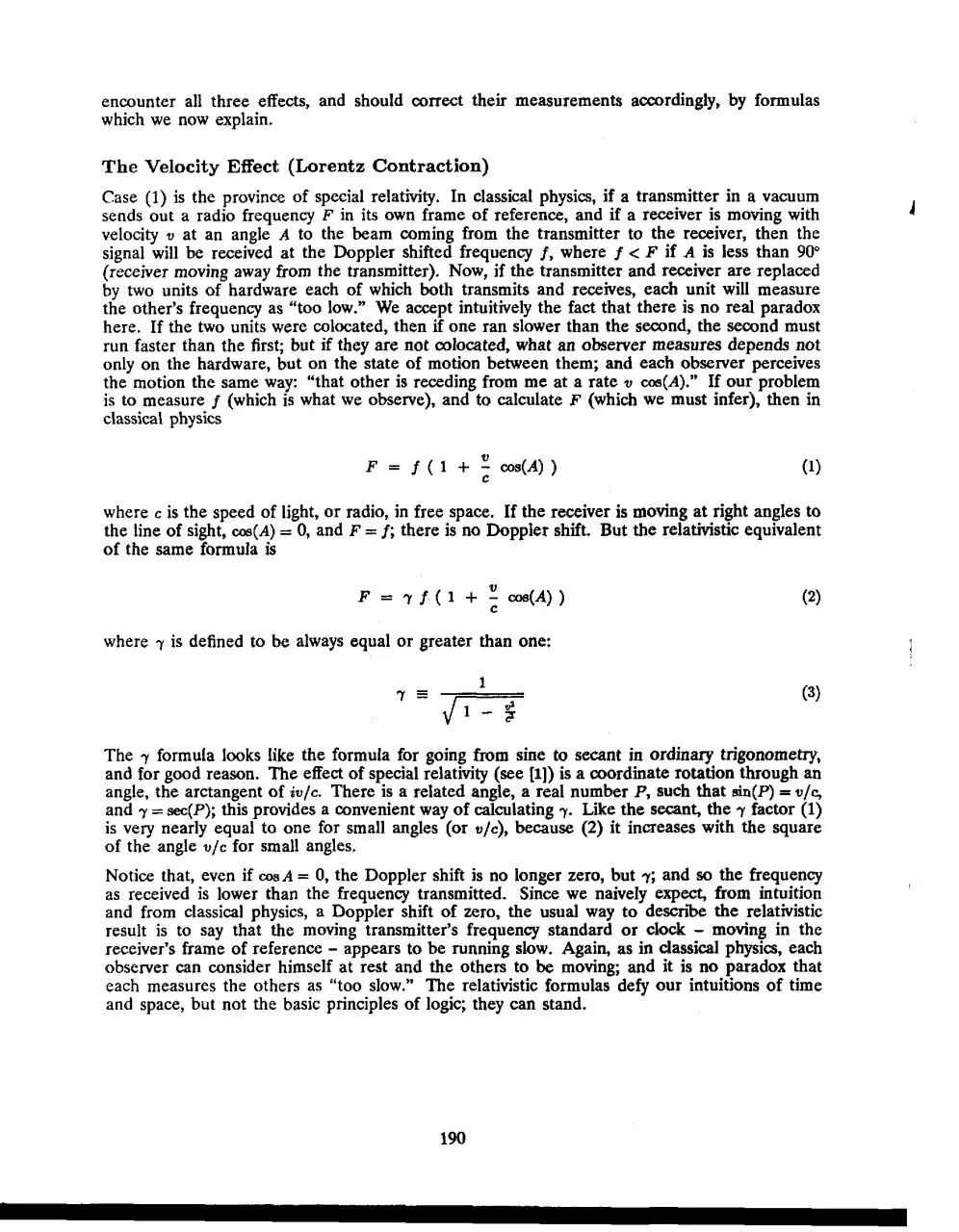
Case (1) is the province of special relativity. In classical physics, if a transmitter in a vacuum
sends out a radio frequency F in its own frame of reference, and if a receiver is moving with
velocity v at an angle A to the beam coming from the transmitter to the receiver, then the
signal will be received at the Doppler shifted frequency f , where f < F if A is less than 90"
(receiver moving away from the transmitter). Now, if the transmitter and receiver are replaced
by two units of hardware each of which both transmits and receives, each unit will measure
the other's frequency as "too low." We accept intuitively the fact that there is no real paradox
here. If the two units were colocated, then if one ran slower than the second, the second must
r
depends not
run faster than the first; but if they are not colocated, what an 0 b S e ~ e measures
only on the hardware, but on the state of motion between them; and each observer perceives
the motion the same way: "that other is receding from me at a rate v cos(A)." If our problem
is to measure f (which is what we observe), and to calculate F (which we must infer), then in
classical physics

1

where c is the speed of light, or radio, in free space. If the receiver is moving at right angles to
the line of sight, -(A) = 0, and F = f; there is no Doppler shift. But the relativistic equivalent
of the same formula is

where

7

is defined to be always equal or greater than one:

The 7 formula looks like the formula for going from sine to secant in ordinary trigonometry,
and for good reason. The effect of special relativity (see [I]) is a coordinate rotation through an
angle, the arctangent of ivlc. There is a related angle, a real number P , such that mn(P) = v / c ,
and 7 = sec(P); this provides a convenient way of calculating 7. Like the secant, the 7 factor (1)
is very nearly equal to one for small angles (or v/c), because (2) it increases with the square
of the angle V / C for small angles.
Notice that, even if cosA = 0, the Doppler shift is no longer zero, but 7; and so the frequency
as received is lower than the frequency transmitted. Since we naively expect, from intuition
and from classical physics, a Doppler shift of zero, the usual way to descriie the relativistic
result is to say that the moving transmitter's frequency standard or clock - moving in the
receiver's frame of reference - appears to be running slow. Again, as in classical physics, each
observer can consider himself at rest and the others to be moving; and it is no paradox that
each measures the others as "too slow." The relativistic formulas defy our intuitions of time
and space, but not the basic principles of logic; they can stand.

4

Now, the angle A should be corrected for aberration. From either a classical or a relativistic
point of view, aberration is the change in the apparent direction from which a wavetrain
appears to be coming because of the observer's velocity. In Eqs. (1) and (2) above, the cosine
of the angle A should be calculated in the observer's frame of reference. If A' is the angle
that is calculated in (for example, the so-called "Earth Centered Inertial" or ECI system of
coordinates, then the relativistic equation to go from cosine of A' to the cosine of A is

and this equation is exact. The reader may wonder why the omnipresent 7 factor does not
appear. It would, in the formulas for sin(A) and tm(A). However, we need ws(A), and the 7
factor cancels out. (For the derivations of all the above equations, see [I].)
So then, to calculate the Doppler correction by which we correct the r e c e ~ e dfrequency from
a GPS satellite - for example, in crosslink ranging from one SV to another - we first calculate
the relative speed of the transmitter to the receiver in the ECI frame, and the angle A' between
relative velocity and the line of sight between transmitter and receiver, also in the ECI frame.
We then apply Eq. (4) to obtain m ( A ) , and then Eqs. (2)-(3) to transform the observed
frequency f to the true transmitted frequency F, in the transmitter's frame of reference.

Gravitational Effect
We now turn to Case (2) above, where the transmitter is higher or lower than the receiver, in
a gravitational field. If a photon (whether of light or of radio) falls into a potential well, it is
shifted to a higher frequency; climbing up, it loses frequency. The quantum acts like a material
particle, gaining kinetic energy as it falls through the gravity field. In quantum mechanics, it is
shown that the energy of the photon is h f , where h is Planck's constant and f is the frequency.
If it were a materiai particle, then from special relativity its total energy would be m 2, where
the kinetic energy is included in the increase of the mass m from the rest mass m. Since h f is
equivalent to m 2, the mass m of the particle must correspond to h f/2 of the photon. Then,
since the change in potential in going from one point to another is the change in energy of
the particle per unit mass, that correspondence requires that

In the earth's gravitational field, if a radio signal passes from a satellite at distance R, from
earth's center to a receiver (whether on another satellite or on the ground) at distance 8,
a good approximation for the frequency shift correction, to transform from the frequency
measured on the ground to the frequency transmitted by the satellite, is

So to the Doppler shift given by Eqs. (Z), (3), and (4) we add the frequency shift from Eq.
(7). If R, is greater than Q, the correction is negative, and so by adding it to the received
frequency f we obtain the frequency F of the transmitter in its own frame of reference.

Acceleration Effect
This is the correction to be made if an observer (= the receiver) is accelerating. In fact, the
receiver, whether in an SV or on the ground, is certainly accelerated; it is either in free fall
in orbit or subject to centripetal acceleration on the rotating earth. Acceleration effect can
be absorbed in the gravity potential. The formal justification for doing so is the Principle of
Equivalence in Einstein's general theory of relativity, which is best explained by an example.
Suppose that a photon of light is radiated across a chamber through a distance r from wall
A to wall B, along a line perpendicular to both walls. Suppose that the whole chamber is
accelerating along this line, in the same direction as the photon is moving, by g meterstsecond
squared. Define the initial velocity as zero at the instant that the photon is radiated; we are
entitled to do this by the principles of special relativity. Now, by the time the photon arrives
at the opposite wall, that wall is receding at a velocity v = -st, where t is r/c, and as measured
by a receiver on the receding wall the photon will be Doppler-downshifted by an amount (in
classical approximation)

But now consider a corresponding scenario in which the chamber is not accelerated, but in
which a gravitational field produces a local acceleration due to gravity, g. As we have seen
(Eqs. (5)-(7) above), the proportional frequency shift is the difference of gravitational potential
divided by c squared. By the Principle of Equivalence, the product gr in Eq. (8) corresponds
to this potential difference, and we can allow for the observer's acceleration by modifying the
gravity term.
But we see that there is no need to do so, if we remember what this modification would be.
The -@/c of Eq. (8) is simply the correction to the Doppler shift due to the change in the
receiver velocity during the signal propagation time - in our example, the time it takes the
photon to traverse ( r ) . But if we compute the Doppler effect by Eq. (Z), using the relative
velocity between transmitter and receiver at the time of reception of the signal, we include the
effect of Eq. (8) automatically. Only if we were to label signal events at the transmission time
would we need to include Eq. (8) explicitly. Among GPS users, hardly anyone does so. If, for
any reason, it is necessary so to do, rewrite Eq. (8) as

where Z is the user's vector acceleration in an inertial frame (e.g, the ECI), and r' is the vector
from transmitter to receiver - at either transmission or reception time, in the "weak field
approximation." This is in the frequency domain; integrate, for timing receivers.

Summary of Corrections T o Be Made
Here is the summary. In general, to correct the frequency measured by a receiver for all
relativistic effects, to obtain the frequency at the transmitter, we perform the following steps.

v

(i) Obtain the velocity of the transmitting satellite, and the velocity u'of the receiver, in an
ECI coordinate frame, for the timcs of reception. Calculate the angle between the receiver's
velocity vector and the line from transmitter to the receiver, in the ECI frame. That is the
angle A' of Eq. (4).
(ii) Apply Eq. (4) to obtain the corresponding angle A in the receiver's frame of reference.
(iii) Calculate the magnitude of the velocity of the GPS satellite with respect to the receiver,
in the ECI frame. That is simply the magnitude of the vector difference C-3. Using Eq. (3),
calculate 7.
(iv) Calculate the Aflf frequency shifts using Eqs. (2) and (7), and add them together. This is
the total correction to be added to the received frequency to obtain the transmitted frequency.
To obtain the correction to add to the transmitted frequency in order to obtain the received
frequency, perform the above steps and reverse the sign. To convert to the time domain,
integrate, and assume any convenient zero of time. Without a timing receiver obsewing four
satellites, one cannot synchronize to GPS time.
Since GPS receivers work in the time and not in the frequency domain, they handle the velocity,
gravity, and acceleration shifts differently than d e d b e d above. First, each GPS space vehicle
(SV) clock is offset from its nominal rate by about -4.45xlO-'O (= -38 microseconds per day)
to allow for the relativistic offsets between the differences between the SV and the ground.
Of this -38 microseconds per day, about -45 are due to the gravitational potential difference
between the SV at its mean distance and the earth's surface, and +7 to the mean SV speed,
which is about 3.87 kmlsec. To this mean correction, each receiver must add a term due to
the eccentricity of the GPS orbit. It can be shown that this effect produces a variation in the
SV clock, as seen from the earth, of

where E? is the vector of position of the SV from the ECI, and ? the velocity vector. This is
the equation given in ICD-GPS-200. It is appropriate for users on or near the earth's surface,
but not users in space, who should apply the frequency correction equations given above, or
their integrals to transform to the time domain.

STICKY WICKETS
We now turn to the misunderstandings that have arisen over the 15 years or so that GPS has
been in operation. Most of the disagreements have semantics for a father. A few arose from
the mathematics of relativity, in going from a rigorous treatment to the approximations that
are found sufficient for the practical use of GPS.
T h e Newtonian World o f the Operational Control S y s t e m
The GPS Operational Control System (GPS) corrects the pseudoranges measured by its Monitor
Stations for the sum of the gravitational and the velocity effects as discussed in the previous
section, but computes the velocity effect only for the mean orbital speed of the satellite, which is
about 3.87 kdsec. The question has been raised: why doesn't the operational s o h a r e calculate
the velocity effect using the speed of each satellite relative to each Monitor Station, which varies

sinusoidally as the Monitor Station is carried around the rotating earth? In principle, it should,
but the effect is negligible for two reasons: (1) the nature of the pseudorange measurement;
and (2) the size of the effect.
The pseudorange measurement can be regarded from two points of view. On the one hand,
pseudorange is simply range, once the clock offsets are removed. As d e s c n i d in the previous
section, the ranges measured by a moving observer are foreshortened by the 7 factor. For an
SV speed of 3.87 kmhec, 7 - 1 is 8.33~10-". The range is typically about 30,000 km. The error
incurred neglecting the q factor is 30,000 km multiplied by 8.33~10-" - that is, 2.5 millimeters.
Close enough for government work.
On the other hand, the pseudorange measurement should be equivalent to accumulated Doppler,
once the ionospheric delays are removed. If the MS accumulated Doppler measurements over
a pass, then, since the OCS assumes Newtonian physics, it would use Eq. (1). In the more
nearly correct world of special relativity, we should use Eq. (2), which differs from Eq. (1)
by the 7 factor. Not only the velocity term, but the observed frequency f , is multiplied by 7.
And 7 is not constant, because the rotation of the earth (up to 0.465 kmlsec at the equator)
vectorially adds to the 3.87 kmlsec of the satellite when we compute the satellite speed relative
to a Monitor Station. Corresponding to a possible v of 3.87 f 0.465 km/sec, 7 can vary from
8.33xlO-"f -1.88~10-". The constant part is absorbed in the mean relativistic offset described
above, but the variable part would alias into the accumulated Doppler range. For example,
over one hour = 3,600 seconds, the error could be 1.88~10-" times 3,600 seconds times c =
20.3 meters. Clearly, this would be a major source of error in the Operational Control System.
But this error would be incurred only if the station clocks were independent of the GPS satellite
clocks, each MS keeping its own time. That's not the way the OCS works. Station time is
estimated in the Kalman filter together with the SV clocks, and each MS clock is effectively
being updated continuously by the satellites. The station clock is used only to bridge the gap in
time between measurements; but since several satellites are always in view, these measurements
are vjrtually instantaneous, except for the different signal propagation times from different
satellites. These times are about 0.1 sec, and, multiplying by 7,once more we derive an error
of about 2.5 millimeters.
However, this happy result depends entirely on the Kalman filter. At present, the filter is very
"springy" - that is, it has a short time constant, because it is adjusted to absorb ephemeris
errors which can change rapidly (for example, at the onset of eclipse). Station clocks, satellite
clocks, and ephemeris parameters are all allowed to move together, and so Monitor Station
time is controlled entirely by the satellite clocks. (If several satellites are in view, the Monitor
Station clock is mathematically redundant, and in practice it drops out of the solution.) But
if the filter were retuned to be very "stiff," with long time constant and reasonable weights
assigned to the Monitor Station clocks, then the appropriate time over which the relativistic
effects would act would no longer nearly equal the signal propagation time, but would be
several hours or days; and then the error due to the neglected 7 factor would approximate that
incurred in the hypothetical accumulated doppler scenario - many meters.
In principle, the critics of GPS in the relativity debate have not been completely wrong. The
neglected 7 factor could hurt us. The OCS software should be reformulated. Nevertheless, in
practice, neglect of relativity does not now contribute measurably to the GPS ermr budget, as
the OCS software is currently configured.

The ECI Coordinate System

I
P

1

I

It has been said (e.g., [?I, and [dl) that the Operational Control System (OCS)of GPS makes
all calculations with respect to an ECI ("Earth Centered Inertial") frame of reference. This
is a perfectly defensible statement, depending on how one chooses to describe the GPS time
scale.
In actual practice, GPS operates in a mixed coordinate system: the spatial coordinates are
ECI, but the time rate is appropriate to observers on the surface of the rotating earth,
that is, in the ECEE GPS time is steered as closely as possible to U.S. Naval Observatory
time (UTCIUSNO]), which in turn is steered closely to International Atomic Time (TAI =
Temps International Atomique). By an important theorem of general relativity, ideal frequency
standards on the rotating geoid run at the same rate, because the effect of the earth's rotation
(by which clocks on the equator would run more slowly than clocks at the poles) is cancelled
by the earth's gravitational potential (since clocks on the equator are farther from the earth's
center, and so at higher potential, than clocks at the poles). So a frequency standard anywhere
on the earth's surface runs at the same rate as one at either pole, and is offset by a constant
rate from a (hypothetical) clock at the earth's center. By the definitions adopted by the
International Astronomical Union (IAU), the ideal time that GPS, UTC, and TAI time scales
realize as nearly as possible is called Terrestrial Time (TT),and the time interval unit of TT is
the Standard International (SI) second on the geoid, also called the coordinate second. Then,
in at least one sense, the time scale of GPS is defined in the ECEF coordinate frame. Also
by Recommendation T1 of the Sub-Group on Time of the IAU Working Group on Reference
Systems, "coordinate times in (a) non-rotating reference system having ... spatial origin at the
geocenter ...(is) designated as Geocentric Coordinate Time (TCG)"; this definition was adopted
by the IAU in its General Assembly in 1991. Therefore, if GPS were to operate in the ECI
coordinate system in the strict sense, its time scale would be TCG, which is offset from TT,
etc. by the potential difference between earth's center and its poles. This GPS does not do.
If a satellite user of GPS were naively to map all measurements "to an ECI frame," using
Geocentric Coordinate Time (TCG), an error would be incurred of roughly 60 microseconds
per day.
However, there is a sense in which the TAI time coordinate is related to the ECI. Although
all ideal frequency standards run at the same rate on the geoid, clocks cannot be synchronized
unless some sort of signals pass between them. Because of the earth's rotation, when clocks
on different continents are compared by travelling frequency standards, satellite signals, or
other means, corrections must be made for the relativistic Sagnac effect. To calculate these
corrections, one must know the rate of the earth's rotation, that is, the angular rate of the
ECEF frame relative to the ECI. Implicitly, then, in the process of forming TAI, to which GPS
time is steered, reference is made to the ECI.

Missing Relativity Terms?
Oversimplifications such as in 141, which disseminated the mistaken notion that GPS time is
calculated "in the ECI," ignoring the earth's rotation, misled Steven Deines, in his paper
entitled, "Uncompensated relativity effects for a ground-based GPS receiver."[sl Deines argued
that
The current ...GPS relativity corrections were based on
an Earth centered inertial reference frame. The derivation
assumed [that] the receiver obtains inertial GPS coordinate

time from the satellites. However, the receiver has been
treated tacitly as being stationary in the inertial frame...
relativity effects for a ground-based receiver include
gravity and Earth rotation. Airborne GPS receivers have
larger effects, and spaceborne GPS receivers have the worst
uncompensated relativity effects.
Deines used equations from Robert Nelson's work (see [6]) in an attempt to show that
corrections depending on the earth's rotation should be added to those incorporated in existing
GPS r e ~ i v e r saccording to ICD-GPS-200. A complete critique of Deines' derivations has been
made by Neil Ashby..Pl Deines overlooked cancellations among several of his terms, by which
the Nelson expressions reduce to very nearly the formulation of ICD-GPS-200.
Nelson shows ([6], p. 21) that the transformation between a time increment dt' expressed in a
rotating andlor linearly accelerated reference frame and a time increment dt in a nonaccelerating
frame is given by

I+.,? + -B( - +dp'G x $ ]

dt = 7 [ l + -

c2

dt'

$dl?

where t? is the acceleration, the position vector of a GPS receiver, v' its velocity, and G the
earth's angular rotation rate. If the ground station is motionless with respect to the earth's
surface, then the acceleration vector @ is determined by 3 and by 8:

and also the velocity ii:

Then one may rewrite Eq. (ll), letting the origin from which p'is measured to be the GPS
receiver, of which the position in ECI coordinates is the vector 8. Eq. (11) now becomes

As Nelson says, terms cancel in Eq. (14) to give a very simple result. The cancellation is as
follows. As is shown in vector algebra,

Therefore, we can write

and Eq. (14) becomes

Eq. (17) "is just what one would expect by a Lorentz transformation from the center of rotation
to the instantaneous rest frame of the accelerated origin" ([6], p. 23). Except for the leading 7
factor, it is the same as the formula derived in classical physics for the signal travel time from
the GPS satellite to the ground station. As we have shown, introducing the y factor makes
a change of only 2 or 3 millimeters to the classical result. In short, there are no "missing
relativity terms." They cancel out.

8 REFERENCES
[I] L. Landau, and E. Lifshitz 1951, The Classical Theory of Fields, trans. M. Hamermesh (Addison-Wesley, Reading, Massachusetts, USA).

[2] P.K. Seidelmann (ed.) 1992, Explanatory Supplement to the Astronomical
Almanac (University Science Books, Mill Valley, California, USA).

[s] N. Ashby, and J J . Spilker, Jr. 1996, "Introduction to relativistic effects on the
Global Positioning System," in Global Positioning System: Theory and Applications, Vol. I, ed. B. Parkinson and J.J. Spilker, Jr. (American Institute of
Aeronautics and Astronautics, Inc., Washington, D.C.. USA)
[4] P.S. Jorgensen 1988-89, "Relativity and intersatellite tracking, * Journal of the
Institute of Navigation, 35, 429ff.
[5] S.D. Deines 1992, "Uncompensated relativity effects for a ground-based GPS receiver, " 0-7803-0468, IEEE.
161

R.A. Nelson 1991, "An analysis of g e n e d ~elativityin the Global Positioning
System time transfer algorithm, " report prepared for Sachflreeman Associates Inc.,
Landover, Maryland, USA.

"Response to Steve Deines' Paper Entitled 'Missing Relativity
Terms in GPS',"University of Colorado, Boulder, Colorado, USA (private communica-

[7] N. Ashby 1996,

tion).
[8] "NAVSTAR GPS Space Segrnent/Navigation User Interfaces, " ICD-GPS-200C,
GPS JPO, 15 Dec 1994.

[s]E. Kaplan (ed.) 1996, Understanding GPS: Principles and Applications (Artech
House, Norwood, Massachusetts, USA).
[lo] MCS software listing obtained from John Berg of the Aerospace Corp., 8 July 1996.
(111

"MAGR Computer Program Development Specification, " XP-RCVR-MAGR, Part

I, 23 Jan 1991.