Econ 5029 exercices2018 (PDF)

ECON 5029 - Carleton University - Exercise set
Professors: Lynda Khalaf and Marcel Voia
Winter 2016
2017
2018
Question 1.
The CAPM was …t, by OLS, (equation by equation) on monthly data from January
1978 to December 1987 for two …nancial assets (CITCRP and MOBIL):
Rit

rf t =

i

+

i

(Rmt

rf t ) + "it ;

"it

i:i:d: 0;

2
i

;

t = 1; :::; T

where, for the month t, Rit is the return on asset i; rf t is the riskless rate of return
and Rmt is the market rate of return. The CAPM assumes that for each asset i = 0:
Estimation results (b i and bi ) are reported in the following Table; OLS standard errors of
estimates are in parentheses (), Newey-West corrected standard errors are in brackets [].
Provide estimates for i and i corrected for contemporaneous correlation of regression
errors; specify the latter hypothesis formally.
Asset
CITCRP

MOBIL

bi
:0025
(:0062)
[:0058]
:0042
(:0059)
[:0051]

bi

:67
(:09)
[:14]
:72
(:09)
[:09]

Question 2
The following model (based on the Phillips curve) is suggested for t = 1; :::; 20 years
and i = 1; 2 (1 = Canada, 2 = U S) countries:
Iti =

i
0

+

i
1 Cti

+ uti

where Iti and Cti are the in‡ation rates and the unemployment rates respectively,
E(uit ) = 0; E(u2it ) =
1

2
i;

E(u1t u2t ) = 0:

Evaluate the following proposition.
Since this model presents grouped heteroskedasticity problems, in order to obtain a
consistent and asymptotically e¢ cient estimate of i0 and i1 , we should apply an appropriate FGLS.
If you approve, explain in details this FGLS and JUSTIFY your answer. Otherwise,
suggest an estimation method that allows us to obtain a consistent and asymptotically
e¢ cient estimate of i0 and i1 .
Question 3.
Consider the system of equations:
Y1t = Xt + e1t ;
; t = 1; :::; T; Xt is non-random
Y2t = + e2t ;
E(e1 ) = 0; V (e1 ) = 1; E(e2 ) = 0; V (e2 ) = 1; E(e1 e02 ) =

12

1. Suppose = 0. Is the OLS estimator of unbiased?
2. Suppose 12 = :5. Explain how you could obtain an e¢ cient estimator of
unconstrained.

for

Question 4.
1. Consider a case where we regress a vector Y on a matrix X by OLS where OLS is
NOT consistent. What is it that OLS is estimating? [Discussion and proof required].
2. Consider a case where we regress a vector Y on a matrix X by OLS where OLS
is consistent. Can this estimator be considered as a special case of Instrumental
Variable (IV) estimation? [Discussion and proof required].
3. Consider a case where we regress a vector Y on a matrix X by OLS where OLS
is consistent, but the regression coe¢ cient is ZERO. Can this estimator (if no
constraints are imposed) produce an EXACT zero as an estimate of the regression
coe¢ cient? [Discussion required].
Question 5.
Equation (33) is proposed based on the Phillips curve for t = 1; :::; 20 years and
i = 1; :::; n countries:
Iit = 0i + 1i Cit + "it
(1)
where Iit and Cit are, respectively, the in‡ation and unemployment rates. Explain in details
how one can obtain asymptotically e¢ cient estimators of the regression coe¢ cients for
ONE of the following two cases:
2

(CASE (A)) n = 10
8i;
1i = 1 8i;
"it = uit + i
E(ui ) = 0; E(ui u0i ) = 2u I20 ; E(ui u0j ) = 0;
0i

where ui is the 20

=

0

1 vector which includes the uit terms, t = 1; :::; 20; and
E( i ) = 0; E( 2i ) =

2

; E(

i j)

= 0:

In addition, i and ui are independent.
(CASE (B)) n = 3 and
V ("it )
COV ("it ; "jt )
COV ("is ; "jt )
COV ("it ; "is )

= 2i 8t;
= ij 8t;
= 0 8t; s
= 0 8t; s:

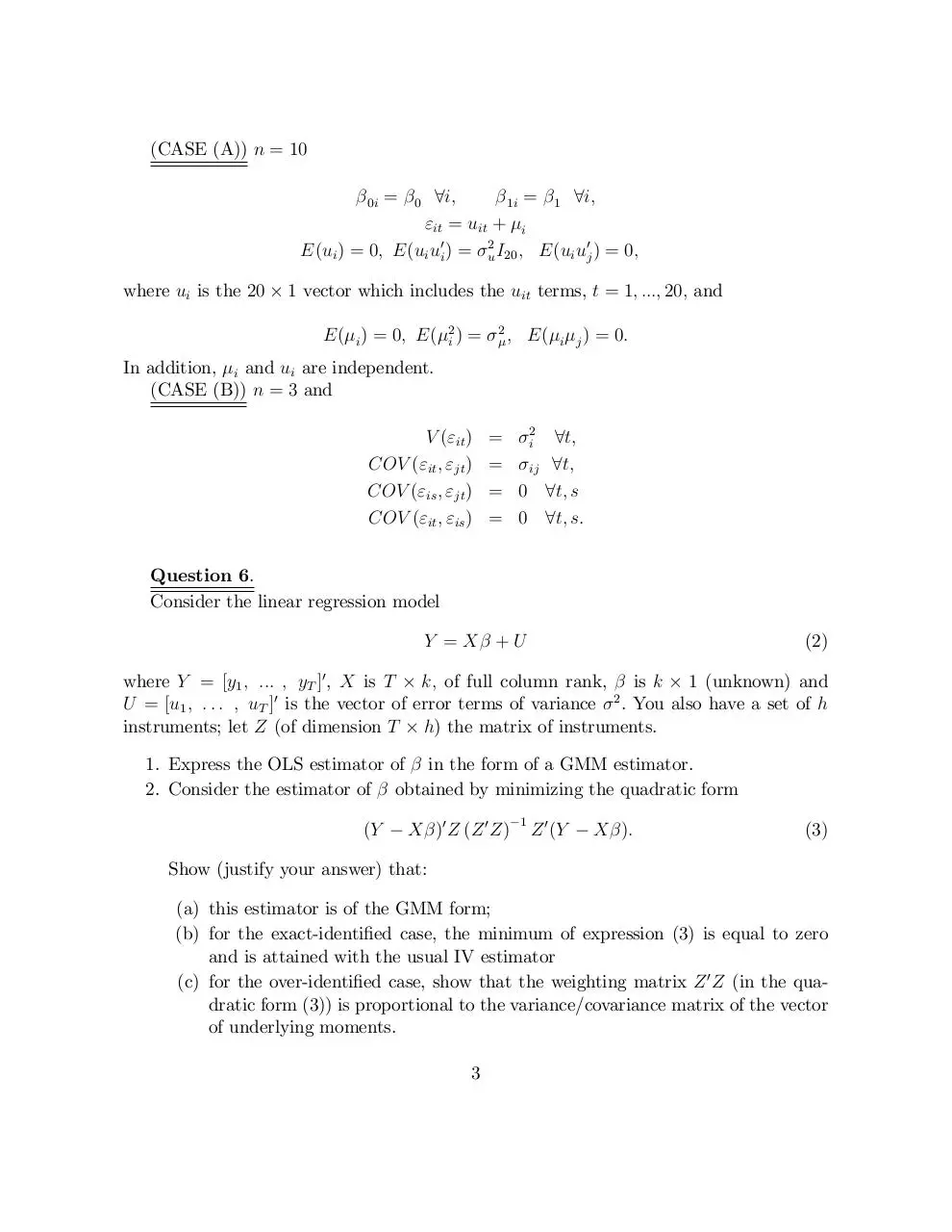
Question 6.
Consider the linear regression model
(2)

Y =X +U

where Y = [y1 ; ::: ; yT ]0 , X is T k; of full column rank, is k 1 (unknown) and
U = [u1 ; : : : ; uT ]0 is the vector of error terms of variance 2 . You also have a set of h
instruments; let Z (of dimension T h) the matrix of instruments.
1. Express the OLS estimator of in the form of a GMM estimator.
2. Consider the estimator of obtained by minimizing the quadratic form
(Y

X )0 Z (Z 0 Z)

1

Z 0 (Y

X ):

(3)

Show (justify your answer) that:
(a) this estimator is of the GMM form;
(b) for the exact-identi…ed case, the minimum of expression (3) is equal to zero
and is attained with the usual IV estimator
(c) for the over-identi…ed case, show that the weighting matrix Z 0 Z (in the quadratic form (3)) is proportional to the variance/covariance matrix of the vector
of underlying moments.
3

Question 7.
A GMM estimator a
^n (of a parameter a) based on the data set Yi ; Xi , i = 1; ::; n; and
a weight matrix Sn ; is typically de…ned as follows:
a
^n = arg min
a

n
P

0

h(Yi ; Xi ; a) Sn

i=1

n
P

h(Yi ; Xi ; a)

i=1

given relevant conditions for the function h(:; a) and the matrix Sn .
1. Show how a moment-matching argument is re‡ected in this objective function
2. How can instruments intervene in the above de…nition?
3. Is it possible that the minimum of the objective function is equal to zero? If yes,
give an example, with proofs.
4. Is it possible that the minimum of the objective function corresponds to an OLS
estimator? If yes, give an example, with proofs.
Question 8.
Consider the following model where i
Cit =

+

1 Yit

+

2 Pit

+

country (N = 10 countries), T = 20 years

3 Vit

+ eit ;

i = 1; : : : ; N;

t = 1; : : : ; T;

Cit
ln(gas consumption, per car, Yit
ln(per capita income),
gas), Vit ln(stock of cars per capita). De…ne
2
3
2
3
C1i
Y1i
6 C2i 7
6
7
7 ; Yi = 6 Y2i 7 ;
Ci = 6
4 :
5
4 :
5
CT i
YT i
2
3
2
3
2
P1i
V1i
1
6 P2i 7
6 V2i 7
6 1
7 ; Vi = 6
7;
6
Pi = 6
n = 4
4 :
5
4 :
5
|{z}
:
n 1
PT i
VT i
1
PT
PT
Cit
Yit
C i = t=1
; Y i = t=1 ;
T
T
PT
PT
P
Vit
it
P i = t=1 ; V i = t=1 :
T
T

Pit

(4)

ln(real price of

3
7
7
5

The following regressions are estimated by OLS, and the residuals are saved in each case.
Regression 1
4

2

3
2
C1
T
6 C2 7
6 T
6
7 on 6
4 :
5
4 :
CN
T
2

C1
6 C2
6
4 :
CN
2

2

3

3

2

C1
6 C2 7
6
6
7 on 6
4 :
5
4
CN
2

C1
6 C2 7
6
6
7 on 6
4 :
5
4
CN

T

3 2

3 2
Y1
P1
7 6 Y2 7 6 P2
7, 6
7 6
5 4 : 5;4 :
YN
PN

Regression 2
3 2
Y1
P1
7
6 Y 2 7 6 P2
7 on N , 6
7;6
5
4 :
5 4 :
YN
PN
3

2

T
T

Y1 P1 V1
0
0
0

3

3
V1
7
6
7
7 and 6 V2 7
5
4 : 5
VN

3

2

3
V1
7
6
7
7 and 6 V 2 7
5
4 :
5
VN

Regression 3
3 2
3 2
Y1
7 6 Y2 7 6
7, 6
7 6
5 4 : 5;4
:
YN
T
Regression 4
0
T Y2 P2 V2
0
0

2

3
2
P1
V1
7
6
P2 7
V2
and 6
5
4
:
:
PN
VN
:
:
:
:

T

YN

3
7
7
5

0
0
0
PN V N

3
7
7
5

1. Can you, if given the outputs of regressions 1-4, obtain SURE-FGLS estimated
for the coe¢ cients of model (4)? If yes, show how. If not, explain why. If more
calculations are needed, explain explicitly what is needed.
2. Can you, if given the outputs of regressions 1-4, obtain a Panel random-coe¢ cients
estimator for the coe¢ cients of model (4)? If yes, show how. If not, explain why. If
more calculations are needed, explain explicitly what is needed.
Question 9.
Consider the following models
case 1: Yit = i Zit + eit i = 1; 2; t = 1; :::; 30 ;
case 2: Yit = i Zt + eit i = 1; 2; t = 1; :::; 30 :
case 3: Yit = Zt + eit i = 1; 2; t = 1; :::; 30
In all cases, the error terms are contemporaneously correlated. Explain how you can obtain
e¢ cient estimates for the coe¢ cients of each model.

5

Question 10.
1. Let (xt ; ) refer a vector of Euler errors of dimension N
1 where xt includes all
data available, is an unknown parameter of dimension of is N
1, and (xt ; )
may be non-linear in variables and in parameters, and can be heteroskedastic and
serially correlated. Setting ft ( ) = ht
(xt ; ), consider a model de…ned by
E(ft ( 0 )) = 0:
2. De…ne the GMM estimator associated with this model and provide an expression
for its asymptotic variance
3. Suppose that the model is linear in variables and in parameters; explain how this
will a¤ect the formulas you provided for the previous two sub-question. In particular, would you have analytical solutions for the point estimator and the standard
errors? If you need further assumptions to obtain analytical solutions, provide them
explicitly.
4. Show how this estimator can be applied to the in‡ation model
t

= st +

=
f

=

b

=

(1

f Et t+1

+

!)(1
)(1
+! ! +!

+!
+!

(5)

b t 1;

! +!
!
! +!

)

(6)

:

provided on pages 5-7 of the lecture notes on GMM. In particular, explain how you
would proceed if you intend to estimate the "reduced form" parameters , f and
and , and if you could assume i.i.d.
b only rather than the "deep parameters" !,
errors.
Question 11.
GMM estimation is motivated by the Law of Large numbers. Suppose that
Yt =

+ Yt

1

+ ut ;

t = 1; :::; T;

where
E(ut ) = 0;
cov(uj ; us ) = 0

V (ut ) =
8j 6= s:
6

2

;

8t

(7)
(8)

Evaluate the following propositions [True, False, Uncertain; proof required]:
1. Since the series Yt , t = 1; :::; T is not i.i.d., then the law of large numbers does
not apply. If you need further assumptions to answer this question, provide them
explicitly.
"
#
T
1X
PLIM
Yt 6= E(Yt ):
T t=1

2. Now assume that

ut = "t ht ; t = 1; :::; T; h2t = 0 + 1 u2t 1 ;
"t
N (0; 1) and "t is independent from ht ;

(9)
(10)

and assess the same proposition for = 0 and 6= 0. If you need further assumptions
to answer this question, provide them explicitly.
Question 12.
Consider the following regression
Yt =

0

+

1 Xt

+ et ; t = 1; : : : ; T

(11)

where Yt = wages, Xt = productivity, in the US for the period 1950-1999 (50 years).
Let b0 and b1 refer to the OLS estimates of 0 and 1 . In the context of the auxiliary
regression
ebt =

ebt

+ error;
b + b Xt ;

1

ebt = Yt

0

(12)

1

let b refer to the OLS estimator de : Suppose that for the data at hand, b = :998 with a
standard error of :002. An econometrician suggest that the latter result provides evidence
in favour of error serial correlation. Another econometrician suggests instead that the
latter evidence signals a spurious regression problem.
1. Apply two tests to assess the claims of both econometricians.
2. Discuss the implications of the test results for the two following cases: (i) DickeyFuller tests on Yt and Xt are signi…cant at the 5% level, and (ii) Dickey-Fuller tests
on Yt and Xt are NOT signi…cant at the 5% level.

7

Question 13.
True, false, Uncertain? (with proof). Propositions 1,2,3 refer to the following model where
Yt crude oil price
Yt = Y t

1

+ et ; t = 2; : : : ; T;

white noise (0;

et

the process has started in an in…nite past and b =

2

) ;

P
Y Y
P t 2t 1 :
Yt 1

1. The error term et
white noise ) A test (at 5% level) for H0 : = 1 can be
obtained based on the student statistic associated with b, by referring the latter
student statistic to a critical point from the student-t distribution.
2. Suppose j j < 1
(a) Yt and Yt k are not correlated for k 1:
(b) et and Yt k are not correlated for k 0:
(c) The regressor Yt 1 is a "lagged endogenous variable" ) b is not consistent.

3. Suppose

=1

(a) A shock that occurs at time t = 2 has a permanent e¤ect on the series.
(b) Any regression that includes Yt on the right hand side will be spurious.

Question 14.
In order to estimate the parameters of a consumption function for the United states,
Ct =

+

Yt + ut ;

t = 1; :::; T;

(1950

93)

you have at hand the following results of several OLS regression [student-t statistics in
parenthesis], where Ct
log(consumptiont ), Yt
log(revenuet ), It
log(investmentt )
and It is exogenous:
Ct\
Ct

1

= 1088:6 + 39:90t
(2:96)

Cbt =

u
bt\
u
bt

1

(2:79)

:1956 Ct

( 2:64)

(13)

1

(14)

65:79 + 0:916Yt

( 0:72)

= 2:940
(0:19)

(2:64)

:207 u
bt ;

( 2:64)

where u
bt = Ct
8

(65:79 + 0:916Yt ) :

(15)

Based on these regressions all estimated by OLS, is the value 0:916 an appropriate
estimate for ? If you have to perform ones or more unit root tests to answer this question,
use a 5% level.
Question 15.
Consider the following regression
Yt = + Y t

+ ut ;

1

(16)

t = 1; :::; T;

where
E(ut ) = 0;
cov(uj ; us ) = 0

V (ut ) =
8j 6= s:

2

;

8t

(17)
(18)

Evaluate the following propositions [proof required].
1. If we assume that Y0 = 0 and = 1, then the variance of Yt is equal to T 2 , where
T is the sample size.
2. If we assume that Y0 = 0 and = 1, then this series cannot …t a TIME TREND
because its expected value does not vary with time.
Question 16
Consider the following model where variables are in deviations from their (sample)
mean, Ct , Yt , It , and rt (consumption, revenue, investment and real interest rate) are
endogenous, Gt (government expenditures) is exogenous:
Ct = 1 Yt + 3 rt + ut
It = 1 rt + 2 Yt 1 + vt
Yt = Ct + It + Gt

(19)
(20)
(21)

1. Study the identi…cation [order condition] of each of the three equations (19), (20)
and (21).
2. 2SLS estimation [using Gt and Yt 1 as instruments] of the equation (19) over 35
years is summarized as follows, with standard errors in parentheses:
bt = :586 Yt
C
(:135)

:00027rt :
(:00076)

Explain in details how this estimation was carried out and how the standard errors
where obtained.
9