The Guggenheim scheme and derivatives thereof (PDF)

The Guggenheim scheme and
derivatives thereof
............
after Edward Armand Guggenheim FRS, 11 August 1901 in Manchester - 9 August 1970

2

1 Introduction
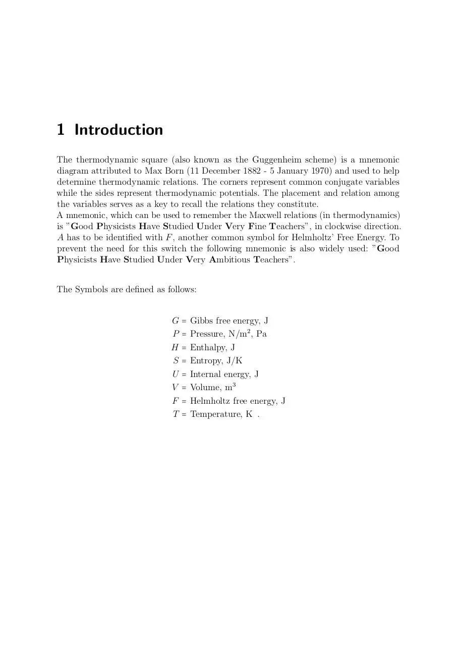
The thermodynamic square (also known as the Guggenheim scheme) is a mnemonic
diagram attributed to Max Born (11 December 1882 - 5 January 1970) and used to help
determine thermodynamic relations. The corners represent common conjugate variables
while the sides represent thermodynamic potentials. The placement and relation among
the variables serves as a key to recall the relations they constitute.
A mnemonic, which can be used to remember the Maxwell relations (in thermodynamics)
is ”Good Physicists Have Studied Under Very Fine Teachers”, in clockwise direction.
A has to be identified with F , another common symbol for Helmholtz’ Free Energy. To
prevent the need for this switch the following mnemonic is also widely used: ”Good
Physicists Have Studied Under Very Ambitious Teachers”.
The Symbols are defined as follows:

G=
P=
H=
S=
U=
V =
F=
T=

Gibbs free energy, J
Pressure, N/m2 , Pa
Enthalpy, J
Entropy, J/K
Internal energy, J
Volume, m3
Helmholtz free energy, J
Temperature, K .

2 Use of the Guggenheim scheme
The Guggenheim scheme is used to compute the derivative of any thermodynamic potential of interest. Suppose for example one desires to compute the derivative of the internal
energy U . The following procedure should be considered:
1. Place yourself in the thermodynamic potential of interest, namely (G, H, U , F ).
In our example, that would be U .
2. The two opposite corners of the potential of interest represent the coefficients
of the overall result. If the coefficient lies on the left hand side of the square, a
negative sign should be added. In our example, an intermediate result would be
dU = −P [Differential] + T [Differential].
3. In the opposite corner of each coefficient, you will find the associated differential.
In our example, the opposite corner to P would be V (Volume) and the opposite
corner for T would be S (Entropy). In our example, an interim result would be:
dU = −P dV + T dS. Notice that the sign convention will affect only the coefficients
and NOT the differentials.
4. Finally, always add the term µ dN , where µ denotes the Chemical potential (also
known as partial molar free energy) in Joule/mole. Therefore, we would have:
dU = −P dV + T dS + µ dN .
The Gibbs-Duhem equation
I

∑ Ni dµi = −S dT + V dP ,
i=1

where Ni is the number of moles of component i, dµi the infinitesimal increase in chemical
potential for this component, S the entropy, T the absolute temperature, V the volume
and P the pressure, can be derived by using this technique. Notice though that the final
addition of the differential of the chemical potential has to be generalized.
The Thermodynamic square can also be used to find the Maxwell Relations. Looking
at the four corners of the square and making a ⊔ shape, one can find ( ∂∂ PS )T = − ( ∂∂ VT )P .
By rotating the ⊔ shape (randomly, for example by 90 degrees counterclockwise into a ⊐
shape) other relations such as: ( ∂∂ PT )V = ( ∂∂ VS )T can be found.
Finally, the potential at the center of each side is a natural function of the variables
at the corner of that side. So, G is a natural function of P and T , and U is a natural
function of S and V .

3 Guggenheim scheme – Derivatives and
further Discussions
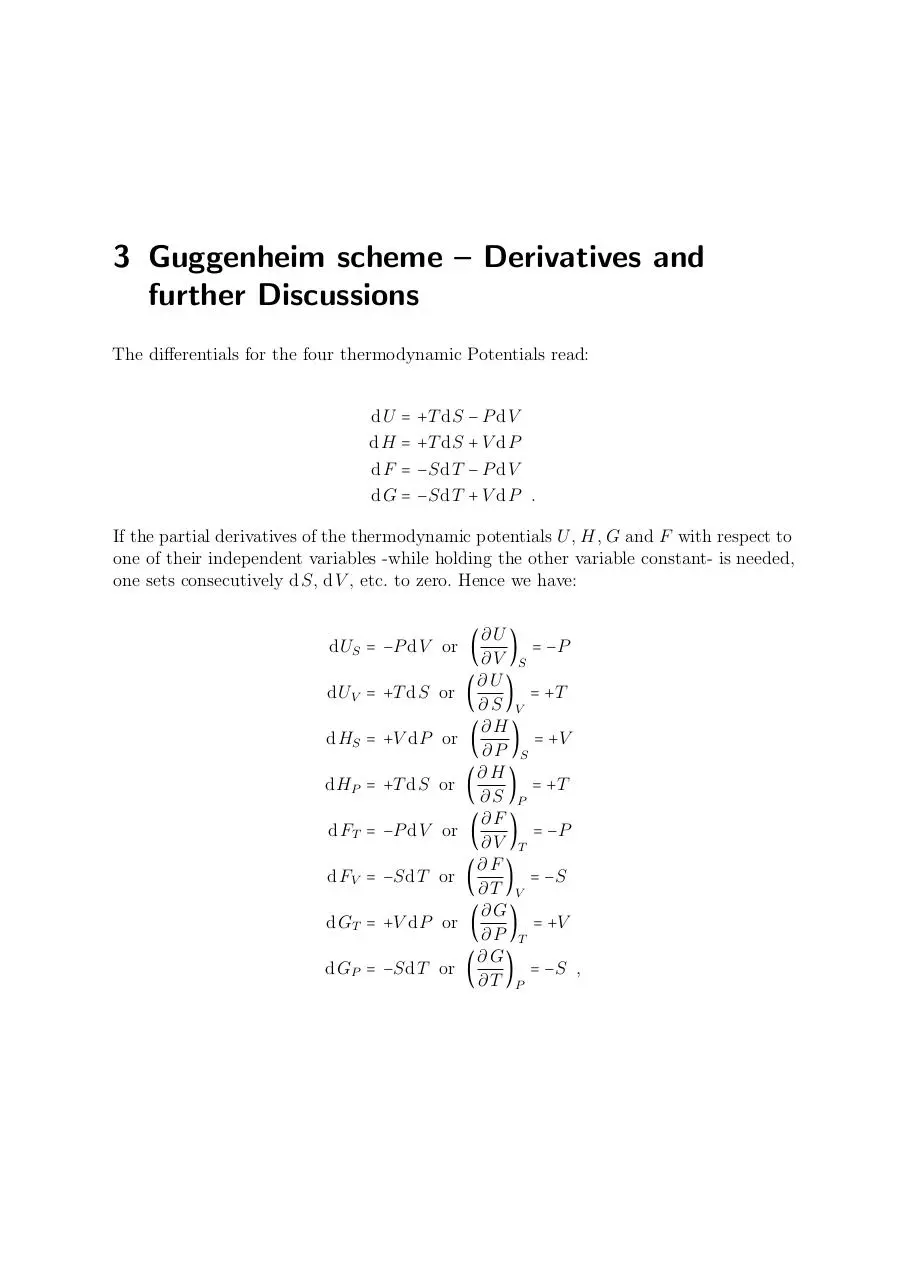
The differentials for the four thermodynamic Potentials read:

dU =
dH =
dF =
dG =

+T dS − P dV
+T dS + V dP
−SdT − P dV
−SdT + V dP .

If the partial derivatives of the thermodynamic potentials U , H, G and F with respect to
one of their independent variables -while holding the other variable constant- is needed,
one sets consecutively dS, dV , etc. to zero. Hence we have:
∂U
) = −P
∂V S
∂U
(
) = +T
∂S V
∂H
(
) = +V
∂P S
∂H
(
) = +T
∂S P
∂F
(
) = −P
∂V T
∂F
(
) = −S
∂T V
∂G
(
) = +V
∂P T
∂G
(
) = −S ,
∂T P

dUS = −P dV or (
dUV = +T dS or
dHS = +V dP or
dHP = +T dS or
dFT = −P dV or
dFV = −SdT or
dGT = +V dP or
dGP = −SdT or

3 Guggenheim scheme – Derivatives and further Discussions

6

which equals, because the partial derivatives have the same values by pairs:
∂U
)
∂S V
∂U
(
)
∂V S
∂H
)
(
∂P S
∂G
(
)
∂T P
(

∂H
) = +T
∂S P
∂F
=(
) = −P
∂V T
∂G
=(
) = +V
∂P T
∂F
=(
) = −S .
∂T V
=(

Three partial derivatives are important in thermodynamics because of their relevance for
important properties of chemicals and the definition for measured variables respectively:
1 ∂V
⋅(
)
V
∂T P
1 ∂V
κ= − ⋅(
)
V
∂P T
∂H
cP = (
)
∂T P
α=

coefficient of isobaric expansion,
coefficient of isothermal compressibility,
specific heat capacity.

So we have three abbreviations α, κ and cP for a differential quotient. These coefficients
have the advantage, that they can be, if applicable, measured with an easy to build
experimental setup or are well known for common substances.
In total, there can be derived from the eight variables U , H, F , G and P , V , T , S 168
partial derivatives (if the reciprocal values are not particularly considered)1 . From these,
some are rarely used if any. But anyway, it would be comfortable, to know all these
partial derivatives without going into detail of the appropriate calculation. It is possible,
to calculate the 168 partial derivatives by rearranging the nominator and denominator
respectively and in this way forming the appropriate quotient. Note, that when the quotient is formed, it is allowed to put only these differentials together, for which the same
variable is to be regarded as constant. However, to perform this calculation and get a
usable result, one has to make reference to some of the derivatives themselves. Three are
1

This subject is called partial permutation. The problem is stated as follows: Given are n
independent elements. How many possibilities exist, to single out k elements out of these n
elements, and to arrange them in a different order? The formula is
Vn,i =

n!
.
(n − k)!

8!
Hence, the result is (8−3)!
= 336, because there are 8 independent thermodynamic potentials (elements) and there are always k = 3 different variables, which form a partial derivative. As the
reciprocal values are not considered, there are 12 ⋅ 336 = 168 possibilities.

3 Guggenheim scheme – Derivatives and further Discussions

7

sufficient and we chose the above mentioned coefficients α, κ and cP , because they are
in most cases readily accessible.
Then, there are 56 of these nominators and denominators necessary for building the
differentials2 . Note, that throughout the following is valid:
(∂ T )P = − (∂ P )T , (∂ V )S = − (∂ S)V , etc.
Hence, we have 56 nominators or denominators, which yields 28 thermodynamic relations
or partial derivatives respectively, which are listed in the box at the end of the chapter.
The above cited abbreviations for α, κ and cP have been used. In the list, there has been
used, if appropriate, the specific heat capacity at constant pressure according to
V T α2
κ
to simplify the result on the r.h.s. of the appropriate equation. Since it follows from
thermodynamical reasoning, that
cP = cV +

∂Q
)
∂T V
and, when V = const. ⇒ −P dV = 0, Q = dU = T dS, because the relation dU = T dS −P dV
holds and according to the second law of thermodynamics Q = T dS, we get
cV = (

cV = (

∂U
) .
∂T V

When we look at the nominator (∂ U )V and the denominator (∂ T )V , we conclude from
the list below, that
(∂ U )V −V ⋅ (κcP − V T α 2 )
=
,
(∂ T )V
−V κ
which simplifies to
cV = cP +
2

V T α2
.
κ

This discipline is called enumerative combinatorics. The problem is stated as follows: Given are
n independent elements. How many various ways exist, to single out k elements out of these n
elements, whereby the sequence of these k elements in the set plays no role but every element k
must be unique in the singled out set? This is calculated as
Cn,i =

n!
,
k! ⋅ (n − k)!

8!
hence, the solution is 3!⋅(8−3)!
= 56, because there are 8 independent thermodynamic potentials
(elements) and we chose k = 3 independent variables α, κ and cP , with which we formulate a
thermodynamic relation, i.e. a partial derivative.

3 Guggenheim scheme – Derivatives and further Discussions

8

This is the just mentioned simplifying equation when we have used cP instead of cV .
It is further possible with the help of the listet formulæ at the end of this chapter to
calculate four partial derivatives for each of the variables α, κ and cP . Again, the nominators and denominators are arranged appropriately, but only these one, for which the
same variable is a constant. One finally gets for α, κ and cP :
∂V
)
∂T P
∂V
(
)
∂G P
∂S
(
)
∂G T
∂S
)
−(
∂P T
(

∂V
)
∂P T
∂V
(
)
∂G T
∂F
−(
)
∂P T
∂F
)
(
∂G T

−(

∂S
)
∂T P
∂S
(
)
∂G P
∂H
(
)
∂T P
∂H
(
)
∂G P
(

=Vα
=−

Vα
S

= −α
=Vα

=Vκ
= −κ
= −P V κ
=Pκ

= cP /T
=−

cP
TS

= cP
=−

cP
.
S

3 Guggenheim scheme – Derivatives and further Discussions

9

The Maxwell relations, as mentioned before, can also be deduced with the help of the
Guggenheim scheme and the list below. The Maxwell relations are named after James
Clerk Maxwell, FRS, (13 June 1831–5 November 1879), who is best known for fusing
magnetism together with electricity into a new field of physics , called electrodynamics,
a classical field theory. The Maxwell relations read as follows:
∂T
)
∂V S
∂T
)
+(
∂P S
∂S
)
+(
∂V T
∂S
−(
)
∂P T
+(

∂P
)
∂S V
∂V
= +(
)
∂S P
∂P
= +(
)
∂T V
∂V
= +(
)
∂T P
= −(

Tα
κcP − V T α 2
V Tα
=
cP
α
=
κ
=

= −V α .

3 Guggenheim scheme – Derivatives and further Discussions

(∂ T )P
(∂ V )P
(∂ S)P
(∂ U )P
(∂ H)P
(∂ G)P
(∂ F )P

= − (∂ P )T = 1
= − (∂ P )V = V α
= − (∂ P )S = cP /T
= − (∂ P )U = cP − P V α
= − (∂ P )H = cP
= − (∂ P )G = −S
= − (∂ P )F = −S − P V α

(∂ V )T
(∂ S)T
(∂ U )T
(∂ H)T
(∂ G)T
(∂ F )T

= − (∂ T )V = V κ
= − (∂ T )S = V α
= − (∂ T )U = V ⋅ (T α − P κ)
= − (∂ T )H = V ⋅ (T α − 1)
= − (∂ T )G = −V
= − (∂ T )F = −P V κ

(∂ S)V = − (∂ V )S = −V ⋅ (κcP /T − V α 2 )
(∂ U )V = − (∂ V )U = −V ⋅ (κcP − V T α 2 )
(∂ H)V = − (∂ V )H = −V ⋅ (κcP − V T α 2 + V α)
(∂ G)V = − (∂ V )G = −V ⋅ (V α − S κ)
(∂ F )V = − (∂ V )F = −V S κ
(∂ U )S = − (∂ S)U = −V P ⋅ (κcP /T − V α 2 )
(∂ H)S = − (∂ S)H = −V cP /T
(∂ G)S = − (∂ S)G = −V ⋅ (cP /T − S α)
(∂ F )S = − (∂ S)F = −V ⋅ (P κcP /T − P V α 2 − S α)
(∂ H)U = − (∂ U )H = V ⋅ (−cP + P V α + P κcP − P V T α 2 )
(∂ G)U = − (∂ U )G = V ⋅ (−cP + P V α + T S α − P S κ)
(∂ F )U = − (∂ U )F = −P V ⋅ (κcP − V T α 2 )
(∂ G)H = − (∂ H)G = −V ⋅ (cP + S − T S α)
(∂ F )H = − (∂ H)F = V ⋅ [(T α − 1) ⋅ (S + P V α) − P κcP ]
(∂ F )G = − (∂ G)F = −V ⋅ (S − P S κ + P V α)

10