lec 15.6up (PDF)

Today.

But first..

Splitting 5 dollars..

This statement is a lie. Neither true nor false!
Every person who doesn’t shave themselves is shaved by the barber.

Finish Counting.
...and then Professor Walrand.

How many ways can Alice, Bob, and Eve split 5 dollars.
Alice gets 3, Bob gets 1, Eve gets 1: (A, A, A, B, E).

Who shaves the barber?

Separate Alice’s dollars from Bob’s and then Bob’s from Eve’s.

def Turing(P):
if Halts(P,P):
while(true):
pass
else:
return

Five dollars are five stars: ? ? ? ? ?.
Alice: 2, Bob: 1, Eve: 2.
Stars and Bars: ? ? | ? | ? ?.
Alice: 0, Bob: 1, Eve: 4.
Stars and Bars: | ? | ? ? ? ?.

...Text of Halt...
Halt Progam =) Turing Program. (P =) Q)
Turing(“Turing”)? Neither halts nor loops! =) No Turing program.
No Turing Program =) No halt program. (¬P =) ¬Q)

Each split “is” a sequence of stars and bars.
Each sequence of stars and bars “is” a split.
Counting Rule: if there is a one-to-one mapping between two
sets they have the same size!

Program is text, so we can pass it to itself,
or refer to self.

Stars and Bars.
How many different 5 star and 2 bar diagrams?
| ? | ? ? ? ?.

7 positions in which to place the 2 bars.
Alice: 0; Bob 1; Eve: 4
| ? | ? ? ? ?.
Bars in first and third position.
Alice: 1; Bob 4; Eve: 0
? | ? ? ? ? |.
Bars in second and seventh position.
7
2
7
2

ways to do so and
ways to split 5 dollars among 3 people.

6 or 7???

Stars and Bars.

An alternative counting.

Ways to add up n numbers to sum to k? or

? ? ? ? ?
Alternative: 6 places “in between” stars.

“ k from n with replacement where order doesn’t matter.”

Each selection of two places “in between” stars maps to an allocation
of dollars to Alice, Bob, and Eve.

In general, k stars n

Ways to choose two different places
ways to choose same place twice
6
2

+ 6 = 21.

7
2

= 21.

6
2
6
1

plus
=6

For splitting among 4 people, this way becomes a mess.
6
3
8
3

+ 2 ⇤ 62 + 61 .
20+ 30 + 6 = 56
.
(8*7*6)/6 = 56.

1 bars.
? ? | ? | · · · | ? ?.

n+k

1 positions from which to choose n

1 bar positions.

✓
◆
n+k 1
n 1
Or: k unordered choices from set of n possibilities with replacement.
Sample with replacement where order doesn’t matter.

Quick review of the basics.

Balls in bins.

Sum Rule
n
···

1
First rule: n1 ⇥ n2 · · · ⇥ n3 .

0

k Samples with replacement from n items: nk .
Sample without replacement: (n n!k )!
Sample without replacement and order doesn’t matter:
“n choose k”

n
k

=

n!
(n k )!k ! .

One-to-one rule: equal in number if one-to-one correspondence.

Combinatorial Proofs.

Theorem:

n
k

=

k +n 1
n

.

“indistinguishable balls” ⌘ “order doesn’t matter”

“only one ball in each bin” ⌘ “without replacement”
5 balls into 10 bins
5 samples from 10 possibilities with replacement
Example: 5 digit numbers.

n k
n
k

How many subsets of size k?
Choose a subset of size n k
and what’s left out is a subset of size k .
Choosing a subset of size k is same
as choosing n k elements to not take.
=) n n k subsets of size k .

52
5

+

52
4

52
3

+

.

Two distinguishable jokers in 54 card deck.
How many 5 card poker hands? Choose 4 cards plus one of 2 jokers!
52
5

+2⇤

52
4

+

52
3

5 indistinguishable balls into 52 bins only one ball in each bin
5 samples from 52 possibilities without replacement
Example: Poker hands.

Wait a minute! Same as choosing 5 cards from 54 or

5 indistinguishable balls into 3 bins
5 samples from 3 possibilities with replacement and no order
Dividing 5 dollars among Alice, Bob and Eve.

Theorem:

Pascal’s Triangle

n

Proof: How many subsets of size k ?

n

1

“k Balls in n bins” ⌘ “k samples from n possibilities.”

Second rule: when order doesn’t matter divide..when possible.

Sample with replacement and order doesn’t matter:

Two indistinguishable jokers in 54 card deck.
How many 5 card poker hands?
Sum rule: Can sum over disjoint sets.
No jokers “exclusive” or One Joker “exclusive” or Two Jokers

3

Foil (4 terms) on steroids:
2n terms: choose 1 or x froom each factor of (1 + x).

Simplify: collect all terms corresponding to x k .
Coefficient of x k is kn : choose k factors where x is in product.

3
0
n +1
k

54
5

=

52
5

+2⇤

52
4

+

52
3

.

Combinatorial Proofs.

0
1 1
1 2 1
1 3 3 1
1 4 6 4 1
Row n: coefficients of (1 + x)n = (1 + x)(1 + x) · · · (1 + x).

Pascal’s rule =)

54
5

=

n
k

2
0

+

1
0
3
1

0
0
2
1

n
k 1

1
1
3
2

.

2
2

1
Theorem: n+
= kn + k n 1 .
k
Proof: How many size k subsets of n + 1?

How many size k subsets of n + 1?
How many contain the first element?
Chose first element, need to choose k
elements.
=) k n 1

.

1 more from remaining n

How many don’t contain the first element ?
Need to choose k elements from remaining n elts.
=) kn
So,

3
3

n +1
k

n
k 1

+

n
k

=

n +1
k

.

Combinatorial Proof.

Theorem:

n
k

=

n 1
k 1

Binomial Theorem: x = 1

+···+

k 1
k 1

.

Proof: Consider size k subset where i is the first element chosen.
{1, . . . , i, . . . , n}

Must choose k 1 elements from n
=) kn 1i such subsets.

i remaining elements.

Add them up to get the total number of subsets of size k
1
which is also n+
k .

Theorem: 2n =

n
n

+

n
n 1

+···+

Simple Inclusion/Exclusion

n
0

Proof: How many subsets of {1, . . . , n}?
Construct a subset with sequence of n choices:
element i is in or is not in the subset: 2 poss.
First rule of counting: 2 ⇥ 2 · · · ⇥ 2 = 2n subsets.

How many subsets of {1, . . . , n}?
n
i ways to choose i elts of {1, . . . , n}.
Sum over i to get total number of subsets..which is also 2n .

Sum Rule: For disjoint sets S and T , |S [ T | = |S| + |T |
Used to reason about all subsets
by adding number of subsets of size 1, 2, 3,. . .
Also reasoned about subsets that contained
or didn’t contain an element. (E.g., first element, first i elements.)
Inclusion/Exclusion Rule: For any S and T ,
|S [ T | = |S| + |T | |S \ T |.

Example: How many 10-digit phone numbers have 7 as their first or
second digit?
S = phone numbers with 7 as first digit.|S| = 109
T = phone numbers with 7 as second digit. |T | = 109 .

S \ T = phone numbers with 7 as first and second digit. |S \ T | = 108 .
Answer: |S| + |T |

Summary.
First Rule of counting: Objects from a sequence of choices:
ni possibilitities for ith choice.
n1 ⇥ n2 ⇥ · · · ⇥ nk objects.

Second Rule of counting: If order does not matter.
Count with order. Divide by number of orderings/sorted object.
Typically: kn .
Stars and Bars: Sample k objects with replacement from n.
Order doesn’t matter.
k 1
Typically: n+
k 1 .
Inclusion/Exclusion: two sets of objects.
Add number of each subtract intersection of sets.
Sum Rule: If disjoint just add.
Combinatorial Proofs: Identity from counting same in two ways.
1
Pascal’s Triangle Example: n+
= k n 1 + kn .
k
RHS: Number of subsets of n + 1 items size k .
LHS: k n 1 counts subsets of n + 1 items with first item.
n
k counts subsets of n + 1 items without first item.
Disjoint – so add!

|S \ T | = 109 + 109

108 .

CS70: Jean Walrand: Lecture 15b.

Key Points

The Magic of Probability
Uncertainty: vague, fuzzy, confusing, scary, hard to think about.

Modeling Uncertainty: Probability Space

I

Uncertainty does not mean “nothing is known”

I

How to best make decisions under uncertainty?
I

1. Key Points

I

2. Random Experiments

I

3. Probability Space
I

Buy stocks
Detect signals (transmitted bits, speech, images, radar,
diseases, etc.)
Control systems (Internet, airplane, robots, self-driving
cars, schedule surgeries in a hospital, etc.)

How to best use ‘artificial’ uncertainty?
I
I

I

Probability: A precise, unambiguous, simple(!) way to think
about uncertainty.

Play games of chance
Design randomized algorithms.

Probability
I
I

Models knowledge about uncertainty
Discovers best way to use that knowledge in making
decisions

Our mission: help you discover the serenity of Probability, i.e., enable
you to think clearly about uncertainty.
Your cost: focused attention and practice on examples and problems.

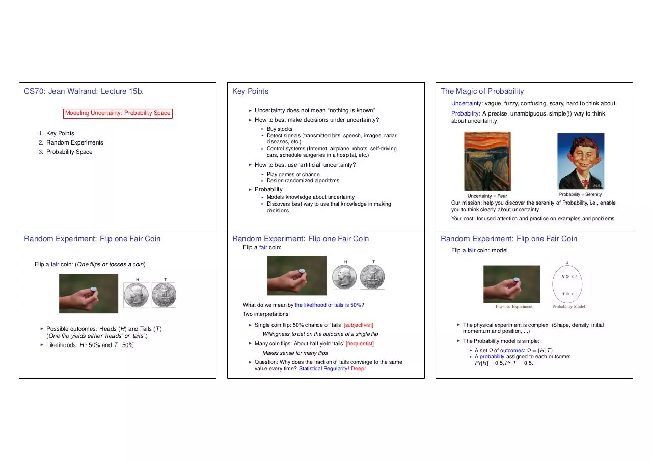
Random Experiment: Flip one Fair Coin

Random Experiment: Flip one Fair Coin
Flip a fair coin:

Random Experiment: Flip one Fair Coin
Flip a fair coin: model

Flip a fair coin: (One flips or tosses a coin)

What do we mean by the likelihood of tails is 50%?
Two interpretations:
I

Possible outcomes: Heads (H) and Tails (T )
(One flip yields either ‘heads’ or ‘tails’.)

I

Likelihoods: H : 50% and T : 50%

I

Single coin flip: 50% chance of ‘tails’ [subjectivist]

I

The physical experiment is complex. (Shape, density, initial
momentum and position, ...)

I

The Probability model is simple:

Willingness to bet on the outcome of a single flip
I

Many coin flips: About half yield ‘tails’ [frequentist]
Makes sense for many flips

I

Question: Why does the fraction of tails converge to the same
value every time? Statistical Regularity! Deep!

I
I

A set ⌦ of outcomes: ⌦ = {H, T }.
A probability assigned to each outcome:
Pr [H] = 0.5, Pr [T ] = 0.5.

Random Experiment: Flip one Unfair Coin

Random Experiment: Flip one Unfair Coin

Flip Two Fair Coins

Flip an unfair (biased, loaded) coin:
I

Flip an unfair (biased, loaded) coin: model

I
I

Possible outcomes: {HH, HT , TH, TT } ⌘ {H, T }2 .

Note: A ⇥ B := {(a, b) | a 2 A, b 2 B} and A2 := A ⇥ A.
Likelihoods: 1/4 each.

p

I

Possible outcomes: Heads (H) and Tails (T )

I

Likelihoods: H : p 2 (0, 1) and T : 1

I

p

Frequentist Interpretation:

Flip many times ) Fraction 1

Physical Experiment

Question: How can one figure out p? Flip many times

I

Tautolgy? No: Statistical regularity!

Flip Glued Coins
Flips two coins glued together side by side:

I
I

Probability Model

p of tails

I

I

1-p

Flip Glued Coins
Flips two coins glued together side by side:

Possible outcomes: {HH, TT }.

I

Likelihoods: HH : 0.5, TT : 0.5.

I

Note: Coins are glued so that they show the same face.

I

Flip two Attached Coins
Flips two coins attached by a spring:

Possible outcomes: {HT , TH}.

I

Likelihoods: HT : 0.5, TH : 0.5.

I

Note: Coins are glued so that they show different faces.

I

Possible outcomes: {HH, HT , TH, TT }.

Likelihoods: HH : 0.4, HT : 0.1, TH : 0.1, TT : 0.4.
Note: Coins are attached so that they tend to show the
same face, unless the spring twists enough.

Flipping Two Coins

Flipping Two Coins

Here is a way to summarize the four random experiments:

Here is a way to summarize the four random experiments:

Flipping n times

Flip a fair coin n times (some n
I

1):

Possible outcomes: {TT · · · T , TT · · · H, . . . , HH · · · H}.
Thus, 2n possible outcomes.

I

I

Note: {TT · · · T , TT · · · H, . . . , HH · · · H} = {H, T }n .

An := {(a1 , . . . , an ) | a1 2 A, . . . , an 2 A}. |An | = |A|n .
Likelihoods: 1/2n each.

Important remarks:
I

Each outcome describes the two coins.

I

⌦ is the set of possible outcomes;

I

E.g., HT is one outcome of the experiment.

I

Each outcome has a probability (likelihood);

I

I

The probabilities are

It is wrong to think that the outcomes are {H, T } and that one
picks twice from that set.

I

Fair coins: [1]; Glued coins: [3], [4];

I

Indeed, this viewpoint misses the relationship between the two
flips.

I

Each w 2 ⌦ describes one outcome of the complete experiment.

0 and add up to 1;

Spring-attached coins: [2];

I

Roll two Dice
Roll a balanced 6-sided die twice:
I
I

Possible outcomes:
{1, 2, 3, 4, 5, 6}2 = {(a, b) | 1  a, b  6}.
Likelihoods: 1/36 for each.

⌦ and the probabilities specify the random experiment.

Probability Space.
1. A “random experiment”:
(a) Flip a biased coin;
(b) Flip two fair coins;
(c) Deal a poker hand.

2. A set of possible outcomes: ⌦.
(a) ⌦ = {H, T };
(b) ⌦ = {HH, HT , TH, TT }; |⌦| = 4;
(c) ⌦ = { A A} A| A~ K , A A} A| A~ Q, . . .}
|⌦| = 52
5 .

3. Assign a probability to each outcome: Pr : ⌦ ! [0, 1].
(a) Pr [H] = p, Pr [T ] = 1 p for some p 2 [0, 1]
(b) Pr [HH] = Pr [HT ] = Pr [TH] = Pr [TT ] = 14
(c) Pr [ A A} A| A~ K  ] = · · · = 1/ 52
5

Probability Space: formalism.
⌦ is the sample space.
w 2 ⌦ is a sample point. (Also called an outcome.)
Sample point w has a probability Pr [w] where
I
I

0  Pr [w]  1;

Âw2⌦ Pr [w] = 1.

Probability Space: Formalism.

Probability Space: Formalism

In a uniform probability space each outcome w is equally
1
probable: Pr [w] = |⌦|
for all w 2 ⌦.

...

Maroon

Physical experiment
I

Flipping two fair coins, dealing a poker hand are uniform
probability spaces.

I

Flipping a biased coin is not a uniform probability space.

Probability Space: Formalism

Simplest physical model of a non-uniform probability space:

[ ]
Red
Green

Examples:

Probability Space: Formalism

Simplest physical model of a uniform probability space:

[ ]

1/8

Red
Green
Yellow
Blue

1/8
...
1/8

Probability model

A bag of identical balls, except for their color (or a label). If the
bag is well shaken, every ball is equally likely to be picked.
⌦ = {white, red, yellow, grey, purple, blue, maroon, green}
1
Pr [blue] = .
8

An important remark

Physical experiment

3/10
4/10
2/10
1/10

Probability model

⌦ = {Red, Green, Yellow, Blue}
3
4
Pr [Red] =
, Pr [Green] =
, etc.
10
10
Note: Probabilities are restricted to rational numbers:

Nk
N .

Lecture 15: Summary

Physical model of a general non-uniform probability space:

[ ]
3

Green = 1
Purple = 2

3

1

...

2

2

Fraction 1
of circumference

Physical experiment

Probability model

The roulette wheel stops in sector w with probability pw .
⌦ = {1, 2, 3, . . . , N}, Pr [w] = pw .

The random experiment selects one and only one outcome
in ⌦.

I

For instance, when we flip a fair coin twice

1
2

...

Yellow

I

I
I

⌦ = {HH, TH, HT , TT }
The experiment selects one of the elements of ⌦.

I

In this case, its would be wrong to think that ⌦ = {H, T }
and that the experiment selects two outcomes.

I

Why? Because this would not describe how the two coin
flips are related to each other.

I

For instance, say we glue the coins side-by-side so that
they face up the same way. Then one gets HH or TT with
probability 50% each. This is not captured by ‘picking two
outcomes.’

Modeling Uncertainty: Probability Space
1. Random Experiment
2. Probability Space: ⌦; Pr [w] 2 [0, 1]; Âw Pr [w] = 1.

3. Uniform Probability Space: Pr [w] = 1/|⌦| for all w 2 ⌦.