deepnorm deep learning (PDF)

DeepNorm - A Deep learning approach to Text
Normalization
Shaurya Rohatgi

Maryam Zare

Pennsylvania State University
State College, Pennsylvania
szr207@ist.psu.edu

Pennsylvania State University
State College, Pennsylvania
muz50@psu.edu

ABSTRACT
This paper presents an simple yet sophisticated approach
to the challenge by Sproat and Jaitly (2016) - given a large
corpus of written text aligned to its normalized spoken form,
train an RNN to learn the correct normalization function.
Text normalization for a token seems very straightforward
without it’s context. But given the context of the used token
and then normalizing becomes tricky for some classes. We
present a novel approach in which the prediction of our
classification algorithm is used by our sequence to sequence
model to predict the normalized text of the input token. Our
approach takes very less time to learn and perform well
unlike what has been reported by Google (5 days on their
GPU cluster). We have achieved an accuracy of 97.62 which
is impressive given the resources we use. Our approach is
using the best of both worlds, gradient boosting - state of
the art in most classification tasks and sequence to sequence
learning - state of the art in machine translation. We present
our experiments and report results with various parameter
settings.

KEYWORDS
encoder-decoder framework, deep learning, text normalization

1

INTRODUCTION

Within the last few years a major shift has taken place in
speech and language technology: the field has been taken
over by deep learning approaches. For example, at a recent
NAACL conference well more than half the papers related in
some way to word embeddings or deep or recurrent neural
networks. This change is surely justified by the impressive
performance gains to be had by deep learning, something
that has been demonstrated in a range of areas from image
processing, handwriting recognition, acoustic modeling in
automatic speech recognition (ASR), parametric speech synthesis for text-to-speech (TTS), machine translation, parsing,
IST 597-003 Fall’17, December 2017, State College, PA, USA
© 2017 Copyright held by the owner/author(s).
ACM ISBN 123-4567-24-567/08/06. . . $15.00
https://doi.org/10.475/123_4

and go playing to name but a few. While various approaches
have been taken and some NN architectures have surely
been carefully designed for the specific task, there is also
a widespread feeling that with deep enough architectures,
and enough data, one can simply feed the data to one’s NN
and have it learn the necessary function. In this paper we
present an example of an application that is unlikely to be
amenable to such a "turn- the-crank" approach. The example
is text normalization, specifically in the sense of a system
that converts from a written representation of a text into a
representation of how that text is to be read aloud. The target applications are TTS and ASR - in the latter case mostly
for generating language modeling data from raw written
text. This problem, while often considered mundane, is in
fact very important, and a major source of degradation of
perceived quality in TTS systems in particular can be traced
to problems with text normalization.
We start by describing the prior work in this area, which
includes use of RNNs in text normalization. We describe the
dataset provided by Google and Kaggle and then we discuss
our approach and experiments 1 we performed with different
Neural Network architectures.

2

RELATED WORK

Text normalization has a long history in speech technology,
dating back to the earliest work on full TTS synthesis (Allen
et al., 1987). Sproat (1996) provided a unifying model for most
text normalization problems in terms of weighted finite-state
transducers (WFSTs). The first work to treat the problem of
text normalization as essentially a language modeling problem was (Sproat et al., 2001 ) . More recent machine learning
work specifically addressed to TTS text normalization include (Sproat, 2010; Roark and Sproat, 2014; Sproat and Hall,
2014).
In the last few years there has been a lot of work that
focuses on social media (Xia et al., 2006; Choudhury et al.,
2007; Kobus et al., 2008; Beaufort et al., 2010; Kaufmann, 2010;
Liu et al., 2011; Pennell and Liu, 2011; Aw and Lee, 2012; Liu et
al., 2012a; Liu et al., 2012b; Hassan and Menezes, 2013; Yang
and Eisenstein, 2013). This work tends to focus on different
problems from those of TTS: on the one hand one, in social
1 https://github.com/shauryr/google_text_normalization

IST 597-003 Fall’17, December 2017, State College, PA, USA

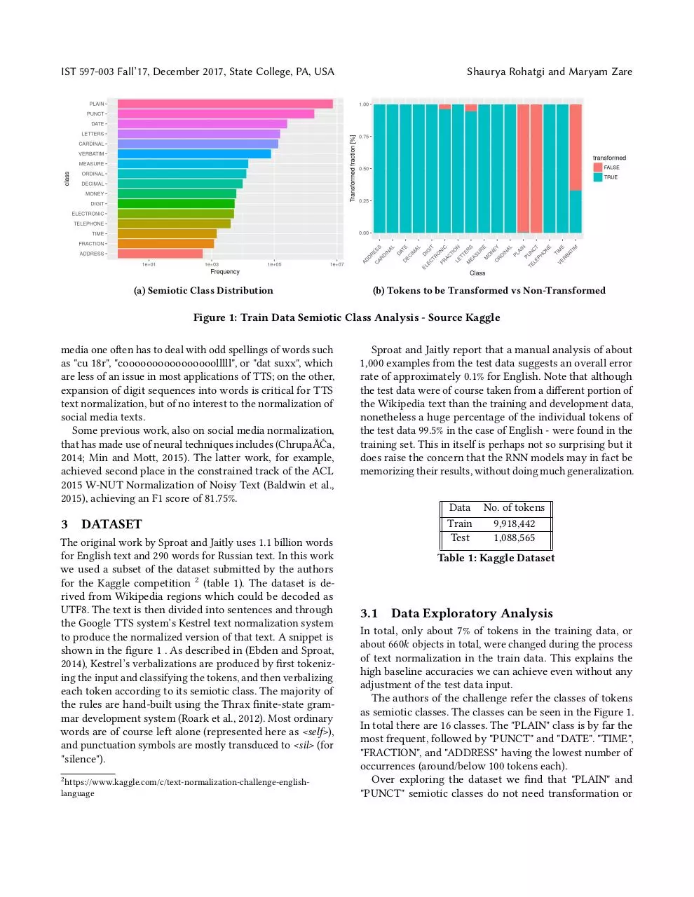
(a) Semiotic Class Distribution

Shaurya Rohatgi and Maryam Zare

(b) Tokens to be Transformed vs Non-Transformed

Figure 1: Train Data Semiotic Class Analysis - Source Kaggle
media one often has to deal with odd spellings of words such
as "cu 18r", "coooooooooooooooolllll", or "dat suxx", which
are less of an issue in most applications of TTS; on the other,
expansion of digit sequences into words is critical for TTS
text normalization, but of no interest to the normalization of
social media texts.
Some previous work, also on social media normalization,
that has made use of neural techniques includes (ChrupaÅĆa,
2014; Min and Mott, 2015). The latter work, for example,
achieved second place in the constrained track of the ACL
2015 W-NUT Normalization of Noisy Text (Baldwin et al.,
2015), achieving an F1 score of 81.75%.

3

Sproat and Jaitly report that a manual analysis of about
1,000 examples from the test data suggests an overall error
rate of approximately 0.1% for English. Note that although
the test data were of course taken from a different portion of
the Wikipedia text than the training and development data,
nonetheless a huge percentage of the individual tokens of
the test data 99.5% in the case of English - were found in the
training set. This in itself is perhaps not so surprising but it
does raise the concern that the RNN models may in fact be
memorizing their results, without doing much generalization.
Data
Train
Test

DATASET

The original work by Sproat and Jaitly uses 1.1 billion words
for English text and 290 words for Russian text. In this work
we used a subset of the dataset submitted by the authors
for the Kaggle competition 2 (table 1). The dataset is derived from Wikipedia regions which could be decoded as
UTF8. The text is then divided into sentences and through
the Google TTS system’s Kestrel text normalization system
to produce the normalized version of that text. A snippet is
shown in the figure 1 . As described in (Ebden and Sproat,
2014), Kestrel’s verbalizations are produced by first tokenizing the input and classifying the tokens, and then verbalizing
each token according to its semiotic class. The majority of
the rules are hand-built using the Thrax finite-state grammar development system (Roark et al., 2012). Most ordinary
words are of course left alone (represented here as <self>),
and punctuation symbols are mostly transduced to <sil> (for
"silence").
2 https://www.kaggle.com/c/text-normalization-challenge-english-

language

No. of tokens
9,918,442
1,088,565

Table 1: Kaggle Dataset

3.1

Data Exploratory Analysis

In total, only about 7% of tokens in the training data, or
about 660k objects in total, were changed during the process
of text normalization in the train data. This explains the
high baseline accuracies we can achieve even without any
adjustment of the test data input.
The authors of the challenge refer the classes of tokens
as semiotic classes. The classes can be seen in the Figure 1.
In total there are 16 classes. The "PLAIN" class is by far the
most frequent, followed by "PUNCT" and "DATE". "TIME",
"FRACTION", and "ADDRESS" having the lowest number of
occurrences (around/below 100 tokens each).
Over exploring the dataset we find that "PLAIN" and
"PUNCT" semiotic classes do not need transformation or

DeepNorm - A Deep learning approach to Text Normalization

IST 597-003 Fall’17, December 2017, State College, PA, USA

Figure 2: Our Model for Kaggle’s Text Normalization Challenge
they need not be normalized. We exploit this fact to our
advantage when we train our sequence to sequence text
normalizer by only feeding the tokens which need normalization. This reduces the burden over our model and filters
out what may be noise for our model. This is not to say that
notable fraction of "PLAIN" class text elements did change.
But the fraction was too less to be considered for training
our model. For example, "mr" to "mister" or "No." to "number".
We also analyzed the length of the tokens to be normalized
in the dataset. We find that short strings are dominant in
our data but longer ones with up to a few 100 characters
can occur. This was common with "ELECTRONIC" class as
it contains URL which can be long.

4

BASELINE

As mentioned above, most of the tokens in the test data are
similar to those in the test data. We exploited this fact to
hold the data in the train set in memory and predicted the
class of the token using the train set.
We have written a set of 16 functions for every semiotic
class to normalize it. Using the predicted class we used the
regular expression functions to normalize the test data. We
understand this is not the correct way to do this, but it provides a very good and competitive baseline for our algorithm.
We score 98.52% on the test data using this approach. This

also defines a line whether our model is better or worse than
memorizing the data.

5

METHODOLOGY

Our approach involves modeling the problem as classification and translation problem. The model has two major parts,
a classifier which determines the tokens that need to be normalized and a sequence to sequence model that normalizes
the non standard tokens (Figure 2). We first explain training
and testing process, then we explain classifier and sequence
to sequence models in more detail.
Figure 2 shows the whole process of training and testing.
We trained classifier and sequence to sequence model individually and in parallel. Training set has 16 classes, 2 of
which don’t need any normalization, so we separated tokens
from those two classes from others and only fed tokens from
remaining 14 classes to the sequence to sequence model. On
the other hand classifier is trained on the whole data set since
it need to distinguish between standard and non standard
tokens.
Once training is done, we have a two stages pipeline ready.
Raw data is fed to the classifier. Results of classifier are two
sets of tokens. Those that don’t need to be normalized are
left alone. Those that need to be normalized are passed to the
sequence to sequence model. Sequence to sequence model
converts the non standard tokens to standard forms. Finally

IST 597-003 Fall’17, December 2017, State College, PA, USA

Shaurya Rohatgi and Maryam Zare

Figure 3: Context Aware Classification Model - XGBoost Semiotic Class Classifier
Window Size Dev Set Accuracy
10
99.8087
20
99.7999
40
99.7841
Table 2: Context aware classification model - Varying
Window size

the output is merged with tokens from the classifier that
were marked as standard ones as the final result.
Now we explain both classifier and normalizer in more detail.

5.1

Context Aware Classification Model
(CAC)

Detecting the semiotic class of the token is the key part
of this task. Once we have determined the class of a token
correctly, we can normalize the it accordingly. The usage
of a token in a sentence determines its semiotic class. To
determine the class of the token in focus, the surrounding
tokens play an important role. Specially in differentiating
between classes like DATE and CARDINAL, for example,
CARDINAL 2016 is normalized as two thousand and sixteen,
while DATE 2016 is twenty sixteen, the surrounding context
is very important.
Our context aware classification model is explained in
the Figure 3 We choose a window size k and we represent
every character in the token with it’s ASCII value. We pad the
empty window with zeros. We use the preceding k characters
of the tokens and the later k characters of the tokens around
the token in focus. This helps the classifier understand in
which context the token in focus has been used. We use
vanilla gradient boosting algorithm without any parameter
tuning. Other experiment details are in the next section.

Figure 4: Sequence to Sequence Model

5.2

Sequence to Sequence Model

In this section we explain the sequence to sequence model
in detail. We used a 2-layer LSTM reader that reads input
tokens, a layer of 256 attentional units, an embedding layer,
and a 2-layer decoder that produces word sequences. We
used Gradient Descent with decay as an optimizer.
The encoder gets the input (x 1 , x 2 , ..., x t 1 ) and decoder gets
the inputs encoded sequence (h 1 , h 2 , ..., ht 1 ) as well as the
previous hidden state st −1 and token yt −1 and outputs (y1 , y2 , ..., yt 2 ).
The following steps are executed by decoder to predict the
next token:
r t = σ (Wr yt −1 + Ur st −1 + Cr c t )
zt = σ (Wz yt −1 + Uz st −1 + Cz c t )
дt = tanh(Wp yt −1 + Up (r t ◦ st −1 ) + Cp c t )

(1)

st = (1 − zt ) ◦ st −1 + zt ◦ дt
yt = σ (Wo yt −1 + Uo st −1 + Co c t )
The model first computes a fixed dimensional representation context vector c t , which is the weighted sum of the
encoded sequence. Reset gate, r, controls how much information from the previous hidden state st −1 is used to create

DeepNorm - A Deep learning approach to Text Normalization

IST 597-003 Fall’17, December 2017, State College, PA, USA

Google’s RNN CAC+Seq2seq
All
0.995
0.9762
PLAIN
0.999
PUNCT
1.00
DATE
1.00
0.998
LETTERS
0.964
0.818
CARDINAL
0.998
0.996
VERBATIM
0.990
0.252
MEASURE
0.979
0.955
ORDINAL
1.00
0.982
DECIMAL
0.995
0.993
ELECTRONIC
1.00
0.133
DIGIT
1.00
0.995
MONEY
0.955
0.824
FRACTION
1.00
0.847
TIME
1.00
0.872
ADDRESS
1.00
0.931
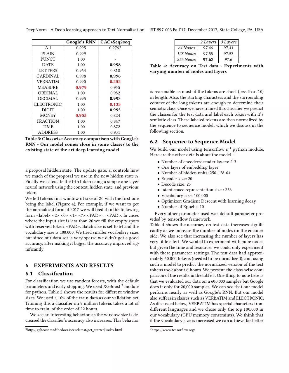
Table 3: Classwise Accuracy comparison with Google’s
RNN - Our model comes close in some classes to the
existing state of the art deep learning model

2 Layers 3 Layers
64 Nodes
97.46
97.41
128 Nodes
97.55
97.53
256 Nodes
97.62
97.6
Table 4: Accuracy on Test data - Experiments with
varying number of nodes and layers

is reasonable as most of the tokens are short (less than 10)
in length. Also, the starting characters and the surrounding
context of the long tokens are enough to determine their
semiotic class. Once we have trained this classifier we predict
the classes for the test data and label each token with it’s
semiotic class. These labeled tokens are then normalized by
the sequence to sequence model, which we discuss in the
following section.

6.2

Sequence to Sequence Model

For classification we use random forests, with the default
parameters and early stopping. We used XGBoost 3 module
for python. Table 2 shows the results for different window
sizes. We used a 10% of the train data as our validation set.
Training this a classifier on 9 million tokens takes a lot of
time to train, of the order of 22 hours.
We see an interesting behavior, as the window size is decreased the classifier’s accuracy also increases. This behavior

We build our model using tensorflow’s 4 python module.
Here are the other details about the model • Number of encoder/decoder layers: 2-3
• One layer of embedding layer
• Number of hidden units: 256-128-64
• Encoder size: 20
• Decode size: 25
• latent space representation size : 256
• Vocabulary size: 100,000
• Optimizer: Gradient Descent with learning decay
• Number of Epochs: 10
Every other parameter used was default parameter provided by tensorflow framework.
Table 4 shows the accuracy on test data increases significantly as we increase the number of nodes on the encoder
side. We also see that increasing the number of layers has
very little effect. We wanted to experiment with more nodes
but given the time and resources we could only experiment
with these parameter settings. The test data had approximately 60,000 tokens (needed to be normalized), and using
such a model to predict the normalized version of the test
tokens took about 6 hours. We present the class-wise comparison of the results in the table 3. One thing to note here is
that we evaluated our data on a 600,000 samples but Google
does it only for 20,000 samples. We can see that our model
performs nearly as well as Google’s RNN. But our model
also suffers in classes such as VERBATIM and ELECTRONIC.
As discussed below, VERBATIM has special characters from
different languages and we chose only the top 100,000 in
our vocabulary (GPU memory constraints). We think that
if the vocabulary size is increased we can achieve far better

3 http://xgboost.readthedocs.io/en/latest/get_started/index.html

4 https://www.tensorflow.org/

a proposal hidden state. The update gate, z, controls how
we much of the proposal we use in the new hidden state st .
Finally we calculate the t-th token using a simple one layer
neural network using the context, hidden state, and previous
token.
We fed tokens in a window of size of 20 with the first one
being the label (Figure 4). For example, if we want to get
the normalized form of 2017 we will feed it in the following
form <label> <2> <0> <1> <7> <PAD> ... <PAD>. In cases
where the input size is less than 20 we fill the empty spots
with reserved token, <PAD>. Batch size is set to 64 and the
vocabulary size is 100,000. We tried smaller vocabulary sizes
but since our data set is very sparse we didn’t get a good
accuracy, after making it bigger the accuracy improved significantly.

6 EXPERIMENTS AND RESULTS
6.1 Classification

IST 597-003 Fall’17, December 2017, State College, PA, USA

Shaurya Rohatgi and Maryam Zare

Semiotic Class
DATE
CARDINAL
DIGIT

before
2016
2016
2016

after (predicted)
twenty sixteen
two thousand and sixteen
two o one six

CARDINAL
TELEPHONE
MONEY

1341833
0-89879-762-4
14 trillion won

one million three hundred fourteen thousand eight hundred thirty three
o sil eight nine eight seven seven sil nine six two sil four
fourteen won

VERBATIM
LETTERS
ELECTRONIC

ω
mdns
www.sports-reference.com

wmsb
cftt
w w r w dot t i s h i s h e n e n e dot c o m

Table 5: Results Analysis of Seq2Seq Model - The prediction gets worse as we go down the table.

results. Also for ELECTRONIC class the window size of the
encoder input was the constraint. We can see from table 5
that it starts well but as the sequence gets longer it predicts
irrelevant characters. We believe increasing the encoder sequence length can improve this aspect of our model.
Table 5 shows the results. For three classes DATE, CARDINAL, and DIGIT the model works very well, and the accuracy
is very close to Google’s model. For example in case of token
’2016’, it is shown that the model can distinguish different
concepts very well and outputs the correct tokens. We think
this is because we are feeding the label with the tokens to
the sequence to sequence model, so it learns the differences
between these classes pretty good.
The next three classes are showing acceptable results. Model
shows some difficulties in telephone numbers, big cardinal
numbers, and class MONEY. Errors are not very bad. In most
cases usually one word is missed or the order is reversed.
We got low accuracy on the last three classes shown in Table
5. We see that Verbatim and Electronic classes have the lowest accuracy. For Verbatim we think the reason is the size
of vocabulary. Since this class consists of special characters
that have low frequency in the data set, a larger vocabulary
could have improve the accuracy a lot. For Electronic class
we think a larger encoder size can be very helpful. This class
has tokens of up to length 40, which don’t fit to the encoder
we used.

7

CONCLUSION

In this project we proposed a model for the task of normalization.We present a context aware classification model and how
we used it to clear out "noisy" samples. We then discuss our
unique model, which at it’s core is a sequence to sequence
model which takes in the label and the input sequence and
predicts the normalized sequence based on the label. We
share our insights and analysis with examples of where our

models shines and where we can improve. We also list out
possible ways of improving the results further. We compare
our results with the state of the art results and show that
given limited computation power we can achieve promising
results This project helped us understand sequence to sequence models and the related classification tasks very well.
We also learned how much parameter tuning can effect the
results and small changes makes big difference. We can also
try Bidirectional RNNs as we saw if the sequence was longer
the model was not accurate.
Finally, we conclude that higher accuracy can be achieved
via having a very good classifier. Classifier has an important
role in this model and there is still lots of room for improvement. Using LSTM instead of XGBoost could have make the
classifier stronger. But we rested our focus mostly on the
sequence to sequence model as we wanted to understand and
implement it. Due to the lack of time and limited resources
we couldn’t try this and we list this as a future work.

REFERENCES
Sproat, R. (1996). Multilingual text analysis for text-to-speech synthesis.
Natural Language Engineering, 2(4), 369-380. Chicago
Sproat, R., Black, A., Chen, S., Kumar, S., Ostendorf, M., & Richards, C.
(1999). Normalization of non-standard words: WS’99 final report. In
Hopkins University.
Sproat, R. (2010, December). Lightly supervised learning of text normalization: Russian number names. In Spoken Language Technology
Workshop (SLT), 2010 IEEE (pp. 436-441). IEEE.
Xia, Y., Wong, K. F., & Li, W. (2006, July). A phonetic-based approach
to Chinese chat text normalization. In Proceedings of the 21st International Conference on Computational Linguistics and the 44th annual
meeting of the Association for Computational Linguistics (pp. 993-1000).
Association for Computational Linguistics.
Choudhury, M., Saraf, R., Jain, V., Mukherjee, A., Sarkar, S., & Basu, A.
(2007). Investigation and modeling of the structure of texting language.
International journal on document analysis and recognition, 10(3), 157174.

DeepNorm - A Deep learning approach to Text Normalization
Marais, K. (2008). The wise translator: reflecting on judgement in translator education. Southern African Linguistics and Applied Language
Studies, 26(4), 471-477.
Kaufmann, M., & Kalita, J. (2010, January). Syntactic normalization of
twitter messages. In International conference on natural language processing, Kharagpur, India.
Clark, E., & Araki, K. (2011). Text normalization in social media: progress,
problems and applications for a pre-processing system of casual English.
Procedia-Social and Behavioral Sciences, 27, 2-11.
Pennell, D., & Liu, Y. (2011, May). Toward text message normalization:
Modeling abbreviation generation. In Acoustics, Speech and Signal
Processing (ICASSP), 2011 IEEE International Conference on (pp. 53645367). IEEE.
Liu, F., Weng, F., & Jiang, X. (2012, July). A broad-coverage normalization system for social media language. In Proceedings of the 50th
Annual Meeting of the Association for Computational Linguistics: Long
Papers-Volume 1 (pp. 1035-1044). Association for Computational Linguistics.
Hassan, H., & Menezes, A. (2013, August). Social Text Normalization
using Contextual Graph Random Walks. In ACL (1) (pp. 1577-1586).
Yang, Y., & Eisenstein, J. (2013, October). A Log-Linear Model for Unsupervised Text Normalization. In EMNLP (pp. 61-72).
ChrupaÅĆa, G. (2014). Normalizing tweets with edit scripts and recurrent neural embeddings. In Proceedings of the 52nd Annual Meeting
of the Association for Computational Linguistics (Vol. 2, pp. 680-686).
Baltimore, Maryland: Association for Computational Linguistics.
Min, W., Leeman-Munk, S. P., Mott, B. W., James, C. L. I., & Cox, J. A.
(2015). U.S. Patent Application No. 14/967,619.
Baldwin, T., de Marneffe, M. C., Han, B., Kim, Y. B., Ritter, A., & Xu,
W. (2015). Shared tasks of the 2015 workshop on noisy user-generated
text: Twitter lexical normalization and named entity recognition. In
Proceedings of the Workshop on Noisy User-generated Text (pp. 126135). Chicago
Sutskever, I., Vinyals, O., & Le, Q. V. (2014). Sequence to sequence learning with neural networks. In Advances in neural information processing
systems (pp. 3104-3112).
Cho, K., Van MerriÃńnboer, B., Gulcehre, C., Bahdanau, D., Bougares,
F., Schwenk, H., & Bengio, Y. (2014). Learning phrase representations
using RNN encoder-decoder for statistical machine translation. arXiv
preprint arXiv:1406.1078.
Chen, T., & Guestrin, C. (2016, August). Xgboost: A scalable tree boosting
system. In Proceedings of the 22nd acm sigkdd international conference
on knowledge discovery and data mining (pp. 785-794). ACM.

IST 597-003 Fall’17, December 2017, State College, PA, USA