Final Image Based Report Mbuvha Wang 2016 .pdf

Convolutional Neural Networks for Distracted
Driver Detection

000
001
002

000
001
002
003

003
004

Rendani Mbuvha, Huijie Wang

004
005

005

KTH Royal Institue of Technology

006

006

007

007

008

008

009

Abstract. In recent years, Convolutional Neural Networks (CNNs) have
become state-of-the-art in Computer Vision. In this work, we apply two
transfer learning methods in solving an image classification problem from
the Kaggle State Farm Distracted Driver Challenge. We show that using off-the-shelf features from pretrained convolutional neural networks
and through fine-turning, high test accuracies of 98.2% and 99.7% are
achieved respectively while training on the full set of subjects. However,
test accuracy severely decreases to 55.9% as training and testing datasets
are split on subjects. As a result, we show the possible overfitting problem which occurs in low-variance datasets and carry out a preliminary
discussion on the reasons behind this. Our best fine tuned model, VGG16 competes relatively well with a Kaggle leaderboard ranking within
the top 20% at the time of submission.

010
011
012
013
014
015
016
017
018
019
020

Keywords: Convolutional Neural Networks; Alexnet; VGG; Transfer
learning; Softmax

022
023

027
028
029
030
031
032
033
034
035
036
037
038
039
040
041
042
043
044

011
012
013
014
015
016
017
018
019
020

022
023
024

024

026

010

021

021

025

009

1

Introduction

The American Centers for Disease Control and Prevention’s (CDC) motor
vehicle safety division has reported that one in five car accidents is caused by a
distracted driver. This translates to approximately 425,000 injuries and 3,000 fatalities caused by distracted driving every year in the United States. Translated
to a global scale this equates to hundreds of thousands of injuries and fatalities annually.In this background, a challenge was step up to help improve these
alarming statistics by State Farm, an American Insurer [1] . This challenge involves solving the image classification problem of identifying driver actions based
on dashboard camera images.
The application of convolutional neural networks (CNNs) in image classification as demonstrated by [2] achieved significantly high accuracy in Large Scale
Visual Recognition Challenge 2012 (ILSVRC2012), this has lead to an explosion
of deep learning research and applications. As deeper and larger convolutional
nets are being applied, the errors on ILSVRC datasets keep decreasing at an
incredible speed, and much research has also endeavoured to find out ways to
transfer such models to various applications, ranging from greenfield projects
such as self-driving cars to classical problems such as speech recognition. As a
result, the authors believe that it is now possible to apply deep convolutional

025
026
027
028
029
030
031
032
033
034
035
036
037
038
039
040
041
042
043
044

2
045
046
047
048
049
050
051
052
053
054
055
056
057
058
059

Rendani Mbuvha, Huijie Wang

neural networks in detecting a driver’s level of distraction with reasonable accuracy.
Pursuant to the above we use transfer learning methods, which takes advantage of pre-trained networks and modifies them to build classifiers suitable for
a specific problem. Two transfer learning approaches are applied in this project
and several popular CNNs are tested, including Alexnet, VGG-F, VGG-M and
VGG-16. The pretrained models are imported from MatConvnet [3]. Methods
in detail including off-the-shelf feature extraction and fine-tuning approaches
will be presented in section 4. Background and related work in image classification and transfer learning will be introduced in section 2. And in section 3, the
dataset from the competition as well as the library used will be described. This
will also include the architectures of the networks we will use. Our experiments
and results will be discussed in section 5 and results will be further compared
and discussed in section 6. Finally, section 7 will make a conclusion about the
project and discuss possible future work.

062
063
064
065
066
067
068
069
070
071
072
073
074
075
076
077
078
079
080
081
082
083
084
085
086
087
088
089

046
047
048
049
050
051
052
053
054
055
056
057
058
059
060

060
061

045

2

Background

Convolutional Neural Networks (CNNs) were first designed in 1968, motivated by animal visual cortex [4] and designed as a feed-forward artificial neural
network. In recent years, CNNs have become a popular method for solving image
classification problems since Krizhevsky et al. won Large Scale Visual Recognition Challenge 2012 (ILSVRC2012) with an eight-layer convolutional neural
network and a top-5 error of 15.3%, this was almost half of the second best
entry’s error at the time [2]. This method was applied on Imagenet, a dataset
including 1.2 million high-resolution images belonging to 1000 classes. From this
success it was found that depth of network significantly influences accuracy. The
model was named Alexnet after the first author. Since then, there has been a
great amount of research in this area, especially on large-scaled deep convolutional networks, due to their high efficiency , flexibility of structure and ease of
training. In the following years of this competition, the accuracy using CNNs
keeps increasing and further proved their ability in image classification problems.
In 2014, VGGNet reduced top-5 error to 7.3% [5] and GoogleLeNet 6.7% [6] .
This two nets go even deeper to reach 16-19 layers and 22 layers respectively.
Further more, the Resnet model reduced error to 3.57% in 2015 with the aid of
152 layers.
From this results it can be seen that CNNs are superior to other models/descriptors for image classification problems due to their large and deep
structures. However, there are several constraints on the training of CNNs. The
first is in the availability of computational resources such as GPU. An typical
example is Alexnet. The model has eight learn-able layers was trained with 60
million parameters and 650 neurons, took several days running using cross-GPU
parallelization. Secondly, the size of training dataset also has decent influence.
Imagenet contains up to 1.3 million images up till now it provides a sufficient representation for various classes of images during training as well as decreases the

061
062
063
064
065
066
067
068
069
070
071
072
073
074
075
076
077
078
079
080
081
082
083
084
085
086
087
088
089

Convolutional Neural Networks for Distracted Driver Detection
090
091
092
093
094
095
096
097
098
099
100
101
102
103
104
105

3

probability of overfitting. As a result, it is resource and time consuming to train
a CNN from scratch. Thus, a more feasible way to avoid such problem is transfer
learning. Several methods are used in transfer learning, such as CNNs fixed feature extractors and fine-tuning the weights of pre-trained networks [7]. Results
from Razavian et al. strongly indicate that off-the-shelf features, i.e. features
obtained from pre-trained CNNs are efficient to be considered as the primary
candidate in most visual recognition tasks [8]. Also Yosinski et al. proved that
using transfer features instead of random initialization not only produces better
performance (even only fine-tuning weights), but also a boost to generalization
[9].
However, although there are some efficiencies using deep learning on classification, there are still no systematic results about the correlations between
accuracy and the structure of the CNNs, including filter size, depth, different
series of layers. In this project, we apply both off-the-shelf feature extraction and
fine-tuning on the distracted driver detection problem and will make discussions
about the performance of different approaches.

3

Dataset and Library

109

3.1

110

The project is taken from the State Farm Distracted Driver Detection [1]
challenge. The learning task in this challenge is to classify driver action based
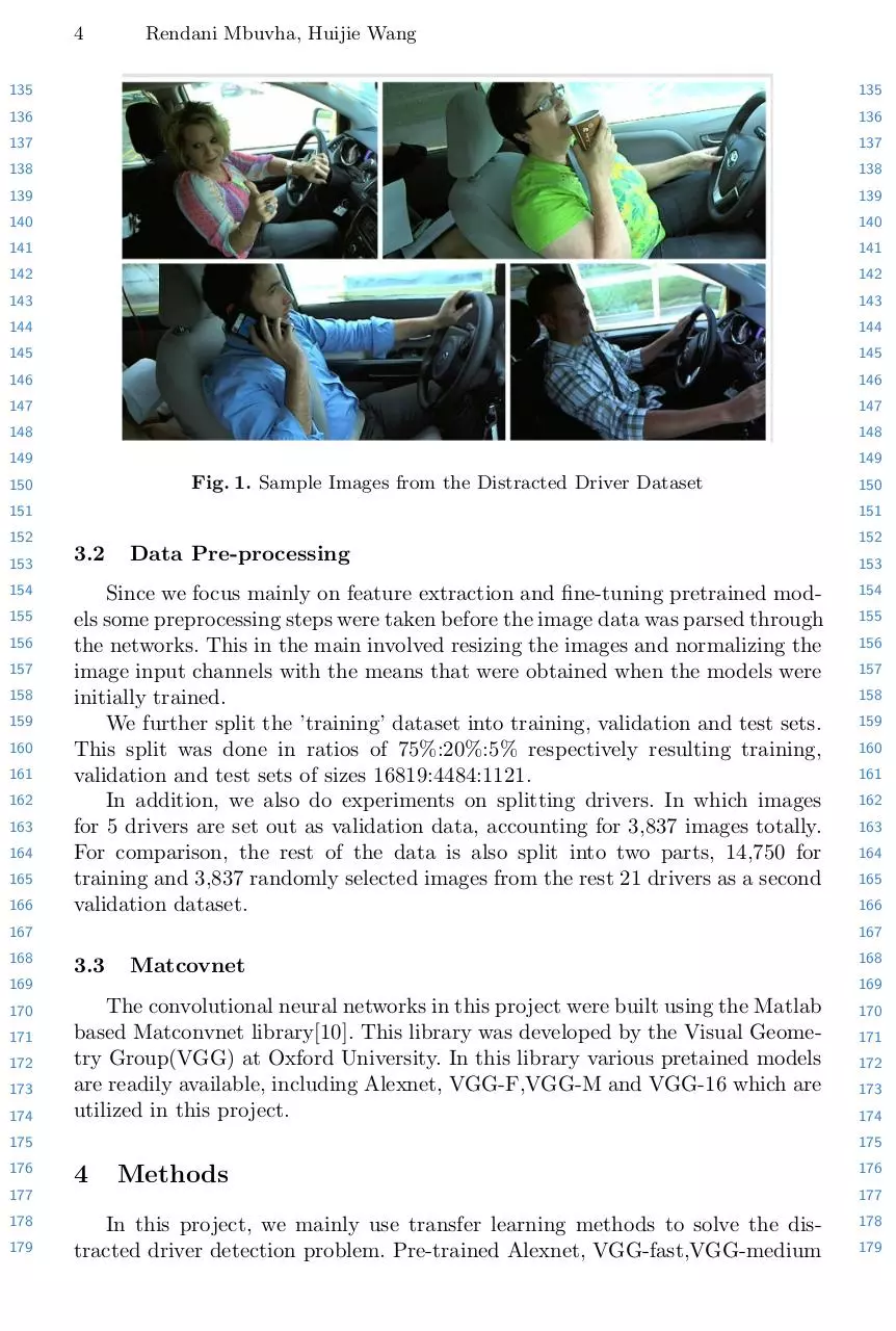
on image data. Two datasets are provided on Kaggle: training and tesing dataset.
The training dataset are labeled and consists of 22,424 480 × 680 RGB dashboard
camera images, with 26 unique drivers performing various actions. These actions
are classified into 10 classes as follows:

112
113
114
115
116
117
118
119
120
121
122
123
124
125
126
127
128
129
130
131
132
133
134

092
093
094
095
096
097
098
099
100
101
102
103
104
105

107
108

108

111

091

106

106
107

090

–
–
–
–
–
–
–
–
–
–

Dataset

c0:
c1:
c2:
c3:
c4:
c5:
c6:
c7:
c8:
c9:

Normal driving
Texting - right
Talking on the phone - right
Texting - left
Talking on the phone - left
Operating the radio
Drinking
Reaching behind
Hair and makeup
Talking to passenger

Figure 1. shows some sample images from this dataset.
On the other hand, Kaggle also provides a testing dataset which contains
79,726 unlabeled images. The two datasets are split on drivers, i.e. a driver can
only appear on either training or testing dataset. This test set is used to evaluate
models submitted by challenge participants.
As Kaggle doesn’t provide naive accuracy for submissions, our experiments
mainly depends on the training dataset, but submission results on Kaggle for
testing dataset is also included. Pre-processing of this dataset will be explained
in Section 3.2.

109
110
111
112
113
114
115
116
117
118
119
120
121
122
123
124
125
126
127
128
129
130
131
132
133
134

4

Rendani Mbuvha, Huijie Wang

135

135

136

136

137

137

138

138

139

139

140

140

141

141

142

142

143

143

144

144

145

145

146

146

147

147

148

148
149

149

Fig. 1. Sample Images from the Distracted Driver Dataset

150

152

152
153
154
155
156
157
158
159
160
161
162
163
164
165
166

3.2

Data Pre-processing

Since we focus mainly on feature extraction and fine-tuning pretrained models some preprocessing steps were taken before the image data was parsed through
the networks. This in the main involved resizing the images and normalizing the
image input channels with the means that were obtained when the models were
initially trained.
We further split the ’training’ dataset into training, validation and test sets.
This split was done in ratios of 75%:20%:5% respectively resulting training,
validation and test sets of sizes 16819:4484:1121.
In addition, we also do experiments on splitting drivers. In which images
for 5 drivers are set out as validation data, accounting for 3,837 images totally.
For comparison, the rest of the data is also split into two parts, 14,750 for
training and 3,837 randomly selected images from the rest 21 drivers as a second
validation dataset.
3.3

Matcovnet

171
172
173
174

The convolutional neural networks in this project were built using the Matlab
based Matconvnet library[10]. This library was developed by the Visual Geometry Group(VGG) at Oxford University. In this library various pretained models
are readily available, including Alexnet, VGG-F,VGG-M and VGG-16 which are
utilized in this project.

4

Methods

179

156
157
158
159
160
161
162
163
164
165
166

168

170
171
172
173
174

176
177

177
178

155

175

175
176

154

169

169
170

153

167

167
168

150
151

151

In this project, we mainly use transfer learning methods to solve the distracted driver detection problem. Pre-trained Alexnet, VGG-fast,VGG-medium

178
179

Convolutional Neural Networks for Distracted Driver Detection
180
181
182

5

and VGG-16 are introduced from Matconvnet [3] and two approaches, off-theshelf and fine-tuning of weights, are applied to this problem. The architectures
of these models are discussed in this section.
4.1

Off-the-shelf feature Extraction from Pretrained CNNs

187
188
189
190
191
192
193
194
195
196
197
198
199

One of the fundamental revelations that has come with the rise of convolutional nets has been the realisation that representations learnt from training a
net for one task can be transferred ’off-the-shelf’ to another task and still give
competitive performance on the new task. [8] show this by performing different
experiments on various object recognition tasks using features extracted from the
first fully connected layer of the overfeat network. Through these experiments
they show that using the above features and a linear SVM classifier outperforms
most of state-of-the-art descriptors.
In our feature extraction experiment we use the representations from the first
fully connected layer of Alexnet [2]. Using these representations which are of 4096
dimensions we train a Softmax classifier with 10 output classes. We perform the
Softmax training using the neural network toolkit in Matlab with 40 ephocs.
The Softmax Classifier is a generalisation of logistic regression for multi-class
classification defined by the function:

200

ex

201

204
205
206
207
208

T

wk

sof tmax(x, k) = PK

xT wk
k=1 e

202
203

for feature vector x and a target class k. The predicted class is then calculated
using the maximum posterior probability.
In training this network we aim to learn the weights wk that minimize the
cross-entropy between the model predictions and the ground truth. The output
of the softmax is posterior probability of the example belonging to class k given
the feature vector x.

211
212
213
214
215

4.2

Fine-tuning the CNNs

We also use fine-tuning method to train our models. In this method, the intial
weights of every layer but last layer are imported from pre-trained models and
20 epochs of learning are applied in order to fine-tune the weights to the current
problem. The detailed structures of the models are discussed in this section.

218
219
220
221
222
223
224

186
187
188
189
190
191
192
193
194
195
196
197
198
199
200
201
202
203
204
205
206
207
208

210
211
212
213
214
215
216

216
217

184

209

209
210

182

185

185
186

181

183

183
184

180

4.3

Architectures

4.3.1 Alexnet Alexnet is a large, deep convolutional neural network which
won Large Scale Visual Recognition Challenge 2012 (ILSVRC2012) [2]. The
structure of Alexnet includes five convolutional layers and three fully-connected
layers. The convolutional layers provide good representation of local features
of image while fully-connected layers mainly learn more general features. As a
result, the size of image is binded due to the fully-connected layers, and here

217
218
219
220
221
222
223
224

6

Rendani Mbuvha, Huijie Wang

225

225

226

226

227

227

228

228

229

229

230

230

231

231

232

232
233

233
234

Fig. 2. Architecture of Alexnet. Figure from [2]

236
237
238
239
240
241
242
243
244
245
246
247
248
249
250
251
252
253
254
255
256
257
258
259

in our project image size is down sampled to 227 × 227 × 3. The structure of
Alexnet is shown in Figure 2.
As it can be seen, each of the linear layers are followed by several normalization layers. In the first three convolutional layers, ReLU, response-normalization
and max-pooling layers are attached. However, the forth convolutional is only
followed by a ReLU layer and the fifth only followed by a ReLU layer and a Pooling layer. The first two fully connected layers are attached with a ReLU layer
and a Dropout layer, with a dropoutrate = 0.5. The dropout layer is used to set
outputs of neurons of the attached hidden layer to zero with a probability of 0.5.
This method not only reduce the computational cost of deep neural network, but
also the complex co-adaption of neurons. As a result, it is an important method
to reduce overfitting problem. The network is fed into a softmax loss regression
for stochastic gradient descent.
In our project, Alexnet is built using the SimpleN N function of MatConvnet.
In order to reduce the training time, the code is rewritten and introduced with
parameters of pre-trained model as initial weights in our network, except for the
last layer, where random weights are created during initialization. This proved
to be more efficient and requires less epochs to converge. The model is trained
using a batch size of 128, following [2], and a learning rate of 0.001, which is
tested to be efficient according to our trials. The size of the output of the last
fully convolutional layer, which acts as a prediction layer, is changed from 1000
to 10 corresponding to our prediction classes. On the other hand, restricted by
computational resources, dense connectivity is used between convolutional layers
instead of the sparse connections used in [2].

262
263
264
265
266
267
268
269

236
237
238
239
240
241
242
243
244
245
246
247
248
249
250
251
252
253
254
255
256
257
258
259
260

260
261

234
235

235

4.3.2 VGG Despite the impressive results achieved by convolutional neural
networks recent years, there is still the non-trivial problem of evaluating how
different structures of CNN perform relative to each other. [11] conducted a
rigorous evaluation on the new techniques, and explored different deep architectures and comparing them on a common ground. Three models, Fast (VGG-F),
Medium (VGG-M) and Slow (VGG-S) are carried out, in which VGG-F is very
similar to Alexnet. On the other hand, VGG-M also has a similar structure but
stride sizes and receptive fields are modified. The first convolutional layer’s stride
size is decreased to 2 (considering that this size is proved to be more suitable

261
262
263
264
265
266
267
268
269

Convolutional Neural Networks for Distracted Driver Detection
270
271
272
273
274
275

7

for Imagenet dataset), while it is increased to 2 in the second layer to limit computation into a reasonable time. On the other hand, the filter size of the first
layer is reduced to 7 × 7 in order to reduce the receptive field. In our project,
VGG-M is implemented using the same method of initialization as Alexnet, as
well as the same parameters of batch size and learning rate. The structures are
shown as Figure 3.

270
271
272
273
274
275

276

276

277

277

278

278

279

279

280

280

281

281

282

282

283

283

284

284

285

285

286

Fig. 3. Architectures of VGG-16. Figure from [11]

286

287

287

288

288

289
290
291
292
293
294

In our project, VGG-F and VGG-M are tested. The depth of VGG was
increased to 16-19 layers during ILSVRC2014 [5]. Limited by computational
resources, we only introduce VGG with 16 layers (VGG-16). The structure of
VGG-16 is shown as Figure 4. It consists of 13 convolutional layers and 3 fullconnected layers. Furthermore, despite the depth, it also differs from Alexnet in
the size of filters are fixed to 3 × 3 and continuous linear layers.

289
290
291
292
293
294

295

295

296

296

297

297

298

298

299

299

300

300

301

301
302

302

Fig. 4. Architectures of VGG nets. Figure elicited from [5]

303

303

304

304

305

305

306

306

307

5

Experiments and Results

309
310
311
312
313
314

307
308

308

5.1

Off-the-shelf features

As described in section 4 our experiments include testing the accuracy of
a softmax classifier trained on features extracted from the first fully connected
layer of Alexnet. The softmax classifier was trained on 16819 training examples
and tested on 1121 unseen examples. The testing performance of the softmax

309
310
311
312
313
314

8

Rendani Mbuvha, Huijie Wang

315

315

316

316

317

317

318

318

319

319

320

320

321

321

322

322

323

323

324

324

325

325

326

326

327

327

328

328

329
330

Fig. 5. Comparison of the confusion matrices for the softmax classifier and a fine turned
Alexnet

332

332

334
335
336
337
338

classifer was compared to that of an Alexnet that was fine-tuned (which will be
discussed in detail in section 5.2) on the same training examples.
Our results are summarized by the confusion matrices in Figure 5.1. We obtain an overall classification accuracies of 98.2% with the off-the-shelf classifier
and 99.7% with the fine tuned CNN on the testing set. However, it should be
mentioned that we achieved 100% accuracy on training data using this approach.
5.2

Fine-tuning on multiple models

343
344
345
346
347
348
349
350
351
352
353
354
355

334
335
336
337
338

340
341

341
342

333

339

339
340

330
331

331

333

329

As shown in the previous section, it is possible that due to the differences
between distracted driver detection dataset and Imagenet, extracting features
directly using pre-trained Imagenet-based model may not have as good performance as fine-tuning. As a result, in this section we focus on fine-tuning based on
Alexnet, VGG-F, VGG-M and VGG-16. It is shown in section 4.3 that VGG-F
has a very similar structure with Alexnet implemented in our project, despite
minor differences of filter depth and numbers. Both of the models have advantage
on training speed from the large stride size of the first convolutional layer. On
the other hand, VGG-M decreases the receptive fields by using smaller filters.
While the stride size of the first two layers are also adjusted. The last CNN we
used, VGG-16 has a relatively different structure with the previous three. The
depth of the net allows it to dig further into image features. And other main
features of VGG-16 lies on fixed filter size (3 × 3) and continuous convolutional
layers.

342
343
344
345
346
347
348
349
350
351
352
353
354
355

356

356

357

357

358

358

359

359

Convolutional Neural Networks for Distracted Driver Detection

9

360

360

361

361

362

362

363

363

364

364

365

365

366

366

367

367

368

368

369

369

370

370

371

371

372

372

373

373

374

374

375

375

376

376

377

377

378

378

379

379

380

(a) Top-1 error rate and energy on training dataset

380

381

381

382

382

383

383

384

384

385

385

386

386

387

387

388

388

389

389

390

390

391

391

392

392

393

393

394

394
395

395
396

(b) Top-1 error rate and energy on validation dataset

398

396
397

397

Fig. 6. Results of fine-tuning

398

399

399

400

400

401

401

402

402

403

403

404

404