05209103 (PDF)
File information
Title: Approximate Equal Frequency Discretization Method
Author: Sheng-yi Jiang, Xia Li, Qi Zheng, Lian-xi Wang
This PDF 1.4 document has been generated by / iTextSharp 4.0.7 (based on iText 2.0.7), and has been sent on pdf-archive.com on 20/10/2017 at 20:05, from IP address 76.118.x.x.
The current document download page has been viewed 345 times.
File size: 252.1 KB (5 pages).
Privacy: public file


File preview
Global Congress on Intelligent Systems
Approximate Equal Frequency Discretization Method
Sheng-yi Jiang, Xia Li, Qi Zheng, Lian-xi Wang
School of Informatics Guangdong University of Foreign Studies Guangzhou 510006 China
jiangshengyi@163.com
There are many classic methods to discretize
continuous
attribute,
including
equal
width
method(EW),equal frequency method(EF),statistic test
method[2-6],information entropy method[7-11] and
clustering-based method[12][13] etc. In general all these
methods use the selected split points to divide the range
of the continuous attribute into finite intervals and label
every interval. These algorithms are categorized as
supervised discretization method and unsupervised
discretization method based on whether it uses class
information or not. This paper studies the method of
unsupervised discretization.
This article is organized as follows. Section 2
introduces equal frequency method and approximate
equal frequency method. Section 3 presents
experimental evaluation with real and synthetic data
sets. Section 4 is the conclusions and directions for
future work.
Abstract
Many algorithms for data mining and machine
learning can only process discrete attributes. In order
to use these algorithms when some attributes are
numeric, the numeric attributes must be discretized.
Because of the prevalent of normal distribution, an
approximate equal frequency discretization method
based on normal distribution is presented. The method
is simple to implement. Computing complexity of this
method is nearly linear with the size of dataset and can
be applied to large size dataset. We compare this
method with some other discretization methods on the
UCI datasets. The experiment result shows that this
unsupervised discretization method is effective and
practicable.
1. Introduction
2.Approximate
Equal
Discretization Method
Discretization is to divide the range of the
continuous attribute into intervals. Every interval is
labeled a discrete value, and then the original data will
be mapped to the discrete values. Discretization of the
continuous attributes is an important preprocessing
approach for data mining and machine learning
algorithm. An effective discretization method not only
can reduce the demand of system memory and improve
the efficiency of data mining and machine learning
algorithm, but also make the knowledge extracted from
the discretized dataset more compact, easy to be
understand and used. Research shows that picking the
best split points is a NP-complete problem[1]. The result
of discretization is related not only with the
discretization algorithm itself but also with the data
distribution and the number of split points. When the
same discretization algorithm is applied to different
dataset, we may get different result. We can only know
the effectiveness of the discretization method by the
result of post processing. So whether the discretization
method is good or not is also related with the induction
algorithm adopted later.
978-0-7695-3571-5/09 $25.00 © 2009 IEEE
DOI 10.1109/GCIS.2009.131
Frequency
2.1 Method Description
Equal frequency method is an unsupervised
discretization algorithm, which tries to put the same
number of values into each interval. If there are n
points in the whole range of the attribute value and we
divide it into k intervals, then every interval will have
n/k points. The equal frequency discretization
algorithm is simple to implement, but due to ignoring
the distribution information of the dataset, the
algorithm can not set interval boundary on the right
position in some situation, so that it doesn’t perform
well. Normal distribution has good characteristic, and it
is also a theoretical basis of many statistic method.
There are many statistic variables in nature science and
behavior science are approximately submission to
normal distribution in large sample. Thus, in this paper
we present an approximate equal frequency
discretization method (AEFD) which based on normal
distribution.
514
to large size dataset, the time complexity of it is less
than that of equal frequency method, PKID
algorithm[17] .
The idea of AEFD is that if a variable is normally
distributed, then the frequency that the observation
value is located in an interval is equal to the probability
that the variable’s value is located in the interval. The
normally distributed variable’s quantile is used to
divide the range of the variable’s value into several
intervals that the variable's value has the same
probability of locating in each interval.
Suppose dividing the range of attribute value into k
intervals: (bi , bi +1 ] (i = 0,1,", k − 1) , b0 = −∞ , bk = ∞ ,
the normally distributed variable has the equal
probability 1/k falling into each of the intervals. After
the discretization, we map every attribute value in
(bi , bi +1 ] (i = 0,1,", k − 1) to a same symbol. AEFD
contains three steps. Details are as follows:
Step1: calculate split points, decide initial dividing
intervals.
Calculate
split
points
according
to
,
here
x
and
σ
is
mean
and
bi = x + Zα ⋅ σ (i = 1,2,", k − 1)
2.3 Further Discussion of the Algorithm AEFD
(1)About the number of the initial divided intervals
k
The number of the initial divided intervals k is
between with ⎡log(n )⎤ and ⎡log(n ) − log(log(n )) ⎤ + 1 , if
⎡log(n ) − log(log(n ))⎤ > 19 , then let k=20. i.e. k is no
more than 20. In latter experiment, we set
k = min{⎡log( n ) − log(log( n ))⎤ + 1,20} .
(2) Condition to merge two intervals
When a interval contains fewer records than a
fraction of the frequency (1/k),MinF, the interval need
to be merged because of its less frequency. MinF can
be set in the range [0.3,0.5]. In our experiment, we set
MinF=1/3.
i
standard deviation of the attribute value, Zα i is the
α i quantile of standard normal distribution ξ ~ N (0,1) ,
(3) Strategy to merge two intervals
There are two different strategies to merge the
objects in the low-frequency interval. The first is to see
the interval as a unit to be merged into the nearest
interval. Second is to merge every object in the interval
one by one into the nearest interval. Considering the
efficiency of the algorithm, we prefer to see the interval
as a whole. Also there are two methods to measure how
close the two intervals are, one is the distance between
the two centroids of the two intervals, the another one
is the distance between the border points of the two
intervals. The experiment shows that the two measure
of the distance of two intervals has almost the same
result. In this paper we use the distance between two
border points of the two intervals.
i
P (ξ ≤ Z α i ) = α i =
( i = 1, 2 , " , k − 1 ) .
k
Via split points we can get the initial k intervals:
(bi , bi +1 ] (i = 0,1,", k − 1) .
Step2: merge the initial divided intervals. That is to
merge the intervals, which contains few records, into
the nearest interval.
Calculate frequency , maximum and minimum of
records
contained
in
every
interval
(bi , bi+1 ] (i = 0,1,2, ", k − 1) ..Searching from right to left,
when the frequency of records contained in
interval (bi , bi+1 ] (i = 0,1,2, ", k − 1) is less than MinF
which is a fraction of frequency (1/k), merge the
interval into its nearest interval and update frequency,
maximum and minimum of records contained in the
interval. The whole process will not stop until no
interval will be merged.
Step3: map values of the continuous attribute into
discrete values with respect to the divided intervals.
(4) Distribution of the data
If we know the distribution of the data, step1 can be
changed to decide the split points based on the given
distribution, and the result will be better.
3. Experimental Results
2.2 Time Complexity of the Algorithm
In order to test the performance of AEFD algorithm,
we select twenty-nine datasets from UCI[15] and a real
salary dataset to be discretized. The character of the
selected datasets is as table 1. Algorithms in Weka
software[16] ,including C4.5, Ripper, Naïve-Bayse
classifer, equal width discretization method (EW),
PKID and supervised discretization method MDL[7],
are used here.
In Step1, operation is fixed, time complexity is
O (1) ; In step2 and step3, we only need to scan the
dataset once to know the objects contained in each
intervals, so time complexity of these two step
is O(n ∗ m) , n is the size of the dataset and m is the
number of the attribute to be discretized. Hence the
whole algorithm need to scan the dataset two times, the
total time complexity is O(n ∗ m) .AEFD can be applied
515
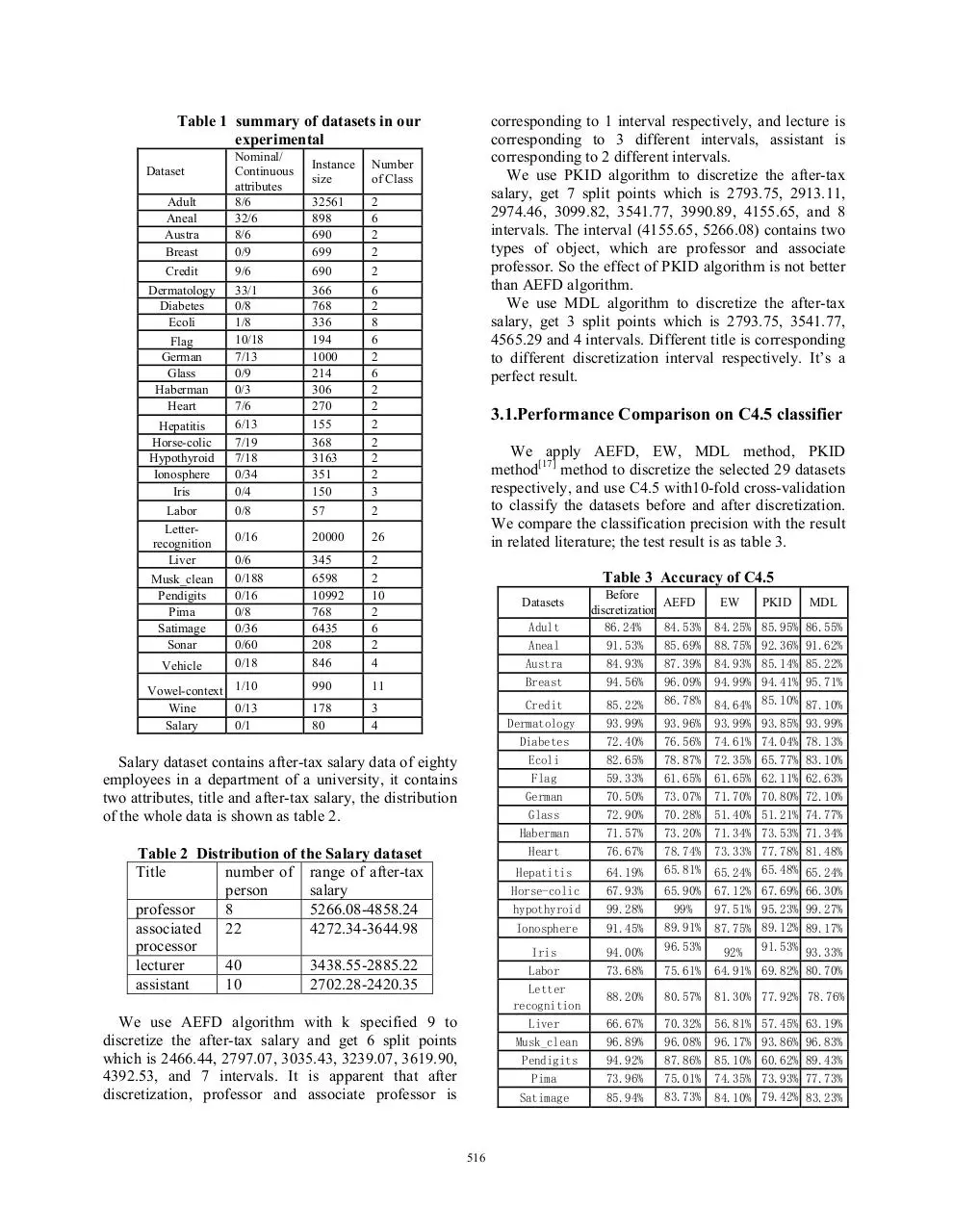
corresponding to 1 interval respectively, and lecture is
corresponding to 3 different intervals, assistant is
corresponding to 2 different intervals.
We use PKID algorithm to discretize the after-tax
salary, get 7 split points which is 2793.75, 2913.11,
2974.46, 3099.82, 3541.77, 3990.89, 4155.65, and 8
intervals. The interval (4155.65, 5266.08) contains two
types of object, which are professor and associate
professor. So the effect of PKID algorithm is not better
than AEFD algorithm.
We use MDL algorithm to discretize the after-tax
salary, get 3 split points which is 2793.75, 3541.77,
4565.29 and 4 intervals. Different title is corresponding
to different discretization interval respectively. It’s a
perfect result.
Table 1 summary of datasets in our
experimental
Dataset
Adult
Aneal
Austra
Breast
Credit
Dermatology
Diabetes
Ecoli
Flag
German
Glass
Haberman
Heart
Hepatitis
Horse-colic
Hypothyroid
Ionosphere
Iris
Labor
Letterrecognition
Liver
Musk_clean
Pendigits
Pima
Satimage
Sonar
Vehicle
Nominal/
Continuous
attributes
8/6
32/6
8/6
0/9
Instance
size
Number
of Class
32561
898
690
699
2
6
2
2
9/6
33/1
0/8
1/8
10/18
7/13
0/9
0/3
7/6
6/13
7/19
7/18
0/34
0/4
0/8
690
366
768
336
194
1000
214
306
270
155
368
3163
351
150
57
2
6
2
8
6
2
6
2
2
2
2
2
2
3
2
0/16
20000
26
0/6
0/188
0/16
0/8
0/36
0/60
0/18
345
6598
10992
768
6435
208
846
2
2
10
2
6
2
4
990
11
178
80
3
4
Vowel-context 1/10
Wine
0/13
Salary
0/1
3.1.Performance Comparison on C4.5 classifier
We apply AEFD, EW, MDL method, PKID
method[17] method to discretize the selected 29 datasets
respectively, and use C4.5 with10-fold cross-validation
to classify the datasets before and after discretization.
We compare the classification precision with the result
in related literature; the test result is as table 3.
Table 3 Accuracy of C4.5
Adult
Aneal
Austra
Breast
Before
discretization
86.24%
91.53%
84.93%
94.56%
Credit
Dermatology
Diabetes
Ecoli
Flag
German
Glass
Haberman
Heart
85.22%
93.99%
72.40%
82.65%
59.33%
70.50%
72.90%
71.57%
76.67%
Datasets
Salary dataset contains after-tax salary data of eighty
employees in a department of a university, it contains
two attributes, title and after-tax salary, the distribution
of the whole data is shown as table 2.
Table 2 Distribution of the Salary dataset
Title
number of range of after-tax
person
salary
professor
8
5266.08-4858.24
associated
22
4272.34-3644.98
processor
lecturer
40
3438.55-2885.22
assistant
10
2702.28-2420.35
We use AEFD algorithm with k specified 9 to
discretize the after-tax salary and get 6 split points
which is 2466.44, 2797.07, 3035.43, 3239.07, 3619.90,
4392.53, and 7 intervals. It is apparent that after
discretization, professor and associate professor is
516
Hepatitis
Horse-colic
hypothyroid
64.19%
67.93%
99.28%
Ionosphere
91.45%
Iris
Labor
Letter
recognition
Liver
Musk_clean
Pendigits
Pima
94.00%
73.68%
Satimage
85.94%
AEFD
EW
PKID
MDL
84.53% 84.25% 85.95% 86.55%
85.69% 88.75% 92.36% 91.62%
87.39% 84.93% 85.14% 85.22%
96.09% 94.99% 94.41% 95.71%
86.78% 84.64% 85.10% 87.10%
93.96% 93.99% 93.85% 93.99%
76.56% 74.61% 74.04% 78.13%
78.87% 72.35% 65.77% 83.10%
61.65% 61.65% 62.11% 62.63%
73.07% 71.70% 70.80% 72.10%
70.28% 51.40% 51.21% 74.77%
73.20% 71.34% 73.53% 71.34%
78.74% 73.33% 77.78% 81.48%
65.81% 65.24% 65.48% 65.24%
65.90% 67.12% 67.69% 66.30%
99%
97.51% 95.23% 99.27%
89.91% 87.75% 89.12% 89.17%
96.53%
92% 91.53% 93.33%
75.61%
64.91% 69.82% 80.70%
88.20%
80.57%
81.30% 77.92% 78.76%
66.67%
96.89%
94.92%
73.96%
70.32% 56.81% 57.45% 63.19%
96.08% 96.17% 93.86% 96.83%
87.86% 85.10% 60.62% 89.43%
75.01% 74.35% 73.93% 77.73%
83.73% 84.10% 79.42% 83.23%
Sonar
Vehicle
Vowel-context
Wine
74.18%
72.72%
80.11%
93.26%
73.03%
68.18%
74.51%
91.29%
69.09%
70.60%
75.05%
78.65%
68.89%
62.25%
49.33%
79.72%
Average
81.37%
80.69%
77.71% 75.67% 81.76%
and after discretization, and compare the classification
precision with the result in related literature; the test
result is as table 5.
80.05%
70.60%
79.23%
94.38%
Table 5 Accuracy of Naïve-Bayes
Before
discretization
Adult
83.38%
Aneal
79.91%
Austra
77.19%
Breast
96.01%
Credit
77.74%
dermatology
97.46%
Diabetes
75.42%
Ecoli
84.88%
Flag
43.35%
German
74.52%
Glass
46.54%
Haberman
74.97%
Heart
84.33%
Hepatitis
69.74%
Horse-colic
67.28%
hypothyroid
97.51%
Ionosphere
82.85%
Iris
95.40%
Data sets
3.2.Performance
classifier
Comparison
on
RIPPER
We randomly disorder the selected 26 datasets ten
times, and apply AEFD, EW, PKID method, MDL
method to discretize them respectively. We use
RIPPER with10-fold cross-validation to classify the
datasets before and after discretization, and compare
the classification precision with the result in related
literature; the test result is as table 4.
Table 4 Accuracy of RIPPER
Data sets
Aneal
Austra
Breast
Credit
Dermatology
Diabetes
Before
discretization
93.58%
84.93%
94.56%
85.22%
88.58%
72.40%
AEFD
EW
PKID
MDL
88.87%
85.64%
95.99%
65.47%
89.75%
74.66%
92.19%
85.25%
93.98%
84.83%
89.51%
73.11%
94.50%
84.99%
93.83%
84.99%
89.73%
74.74%
94.55%
86.01%
95.26%
86.64%
88.33%
77.51%
Ecoli
Flag
German
Glass
Haberman
82.23%
59.90%
70.50%
72.90%
72.81%
79.52%
62.89%
71.24%
63.22%
75.20%
74.85%
61.65%
69.86%
50.19%
73.33%
78.69%
62.58%
70.15%
60.42%
72.25%
82.26%
61.70%
71.91%
70.65%
72.12%
Heart
Hepatitis
Horse-colic
Hypothyroid
Ionosphere
Iris
76.67%
62.97%
67.93%
99.16%
91.45%
94.00%
80.04%
70.06%
84.59%
98.96%
90.10%
95.47%
78.26%
69.10%
84.62%
97.19%
87.44%
92.53%
78.89&
69.74%
72.20%
97.72%
88.69%
92.60%
82.33%
68.07%
86.09%
99.14%
91.74%
94.87%
Labor
Liver
Pendigits
Pima
Satimage
Sonar
Vehicle
vowel-context
Wine
Average
73.68%
66.67%
94.27%
73.96%
85.79%
74.71%
68.91%
70.64%
93.26%
79.68%
83.33%
63.80%
90.37%
74.79%
82.32%
70.91%
64.11%
65.29%
89.66%
79.09%
83.51%
62.09%
89.44%
74.01%
83.40%
66.88%
63.42%
66.65%
83.99%
78.13%
80.70%
54.84%
82.46%
74.05%
76.30%
57.50%
58.39%
43.41%
90.00%
76.22%
87.02%
63.19%
90.46%
77.30%
83.56%
79.18%
67.74%
73.62%
94.66%
81.77%
AEFD
EW
PKID
MDL
82.58%
90.38%
86.06%
97.32%
85.78%
97.90%
75.47%
83.78%
59.59%
75.12%
64.02%
75.95%
84.07%
68.58%
68.91%
98.24%
89.15%
94.73%
81.86%
92.17%
85.29%
97.25%
84.81%
97.68%
75.36%
80.51%
59.38%
75.43%
57.01%
75.26%
83.30%
68.28%
68.97%
96.87%
90.51%
94.13%
83.75%
95.81%
86.42%
97.25%
85.67%
97.46%
73.54%
80.71%
59.95%
74.78%
65.00%
72.06%
81.81%
67.35%
69.84%
97.62%
88.15%
92.60%
83.88%
95.79%
85.65%
97.22%
86.23%
97.89%
77.92%
85.77%
59.23%
74.67%
72.34%
72.55%
83.04%
71.10%
66.44%
98.60%
90.94%
94.47%
Labor
Letter
recognition
Liver
Musk_clean
91.93%
92.11% 92.81% 91.93% 93.51%
64.14%
72.33% 69.78% 73.21% 73.72%
55.77%
83.76%
64.96% 64.12% 62.26% 63.19%
79.68% 79.81% 90.96% 91.56%
Pendigits
80.37%
85.98% 85.63% 85.45% 87.18%
Pima
73.45%
74.49% 74.26% 72.04% 77.28%
Satimage
Sonar
Vehicle
Vowel-context
Wine
Average
79.55%
68.17%
44.53%
61.89%
96.85%
76.17%
81.61%
75.96%
58.44%
62.55%
97.36%
80.11%
80.59%
75.91%
60.07%
62.37%
96.35%
79.51%
82.18%
72.55%
61.02%
55.72%
95.06%
79.73%
82.23%
85.10%
62.07%
64.19%
98.88%
81.82%
The experiment result shows that the classification
precision after AEFD discretize preprocessing is higher
than that after the preprocessing by EW, PKID method
in the most situation. In close to fifty percent situations,
the
classification
precision
after
discretize
preprocessing by AEFD is better than thatbefore
discretize preprocessing and close to the classic
supervised discretization algorithm MDL.
4. Conclusion
AEFD algorithm is based on normal distribution
theory and notices that the large samples of real data is
approximately submission to normal distribution. The
algorithm is simple, without complicated theory, and
easy to understand and implement. The algorithm has
nearly linear time complexity and the experimental
results show that the AEFD is better than the previous
3.3. Performance Comparison on Naïve-Bayes
Classifier
We randomly disorder the selected 29 datasets ten
times, and apply AEFD, EW, PKID method, MDL
method to discretize them. We use Naïve-Bayes with
3-fold cross-validation to classify the datasets before
517
unsupervised discretization algorithm. Similar to EF
method, AEFD does not fully consider the data’s
distribution information. In some situations, it can not
set the interval border on the properest position. The
further work is to find method that can recognize
intervals of one dimension data with different
distribution density, and further to find the nature
discrete intervals to improve discretization result.
[11] Chang-Hwan Lee. A Hellinger-based discretization
method for numeric attributes in classification learning.
Knowledge-Based Systems. 2007,20(4): 419-425.
[12]LI Xing-sheng,LI De-yi.A New Method Based on
Density Clustering for Discretization of Continuous
Attributes[J].Acta Simulata Systematica Sinica.
2003.6:804-806.
[13]XI Jing,OUYANG Wei min.Clustering Based Algorithm
for Best Discretizing Continuous Valued Attributes[J].
Mini-micro systems. 2000,21 (10):1025-1027
[14]Dougherty J R, Kohavi, Sahami M. Supervised and
Unsupervised Discretization of Continuous Features.
Machine Learning[A] .Proc of 12th International
Conference, Morgan Kaufmann[C].1995:194-202
[15] Asuncion, A. & Newman, D.J. UCI Machine
Acknowledgments
This work is supported by the National Natural Science
Foundation of China (No.60673191), the Natural
Science Research Programs of Guangdong Province’s
Institutes of Higher Education (No.06Z012) and
Guangdong University of Foreign Studies Team
Research Program of Innovations (No.GW2006-TA005).
Learning
Repository
[http://www.ics.uci.edu/~mlearn/MLRepository.ht
ml]. 2007.
[16] weka. http://www.cs.waikato.ac.nz/ml/weka/
[17]Y Yang, GI Webb.A Comparative Study of
Discretization
Methods
for
Naive-Bayes
Classifiers.Pacific
Rim
Knowledge
Acquisition
Workshop (PKAW'02), Tokyo, 2002: 159-173
References
[1] H.S.Nguyen,A.Skowron.Quantization of Real Values
Attributes Rough Set and Boolean Reasoning
Approaches[A].Proc. of the 2th joint Annual Conf on
Information
Sci[C].USA
Wrightsville
Beach,NC,1995:34-37.
[2] Kerber R. Discretization of Numeric Attributes [A]. The
9th International Conference on Artificial Intelligence
[C].1992.
[3] Liu H, Setiono R. Feature selection via discretization[J].
IEEE Transactions on Know ledge and Data
Engineering, 1997, 9(4):642-645.
[4] Tay E H, Shen L. A modified Chi2 algorithm for
discretization[J].IEEE Transactions on Knowledge and
Data Engineering,2002,14(3):666-670.
[5] LI Gang,TONG Fu.An Unsupervised Discretization
Algorithm Based on Mixture Probabilistic Model[j].
Chinese Journal of Computers, 2002,25(2):158- 164
[6]I. Kononenko. Inductive and bayesian learning in medical
diagnosis[J].Applied Artificial Intelligence.1993,7:317–
337.
[7] Fayyad U M,Irani K B.Multi-interval discretization of
continuous valued attributes for classification
learning[A]. Proc. of the 13th International Joint
Conference on Artificial Intelligence[C],1993:10221029.
[8] Clarke EJ,Braton BA.Entropy and MDL discretization of
continuous variables for Bayesian belief networks[J].
International Journal of Intelligence Systems,
2000,15:61-92.
[9] Chiu D K Y, Cheng B, Wong A K C. Information
Synthesis Based on Hierarchical Maximum Entropy
Discretization.Journal of Experimental and Theoretical
Artificial Intelligence,1990,2:117-129.
[10] XIE Hong,CHENG Hao-Zhong, NIU dong-Xiao.
Discretization of Continuous Attributes in Rough Set[J].
, Chinese Journal of Computers, 2005,28(9):1570-1574.
518
Download 05209103
05209103.pdf (PDF, 252.1 KB)
Download PDF
Share this file on social networks
Link to this page
Permanent link
Use the permanent link to the download page to share your document on Facebook, Twitter, LinkedIn, or directly with a contact by e-Mail, Messenger, Whatsapp, Line..
Short link
Use the short link to share your document on Twitter or by text message (SMS)
HTML Code
Copy the following HTML code to share your document on a Website or Blog
QR Code to this page

This file has been shared publicly by a user of PDF Archive.
Document ID: 0000687490.