Exules (PDF)

Exules
Hammad Rana
Abstract: This paper will be dedicated to establishing the concept of exules. The term exul (singular for
exules) means exile in Latin. So in a sense an exul is essentially the exiled data from a geometric
structure that is not discovered from conventional (differential or algebraic) geometric tools. We
will use categories and model theory as our main tools to inspect exules. Exules of polynomials
will serve as the main and initial concept we are interested in exploring but we will also go over
exules of manifolds and other kinds of structures. The final talk will be on generalizing the
concept of exules to work with any mathematical structure.

1
1.1

Exules over Polynomials
Equation of a circle

Suppose we have a multivariate polynomial function
that represents the equation of the circle, centered at
(0,0).
(1)
Z = X 2 + Y 2 = R2
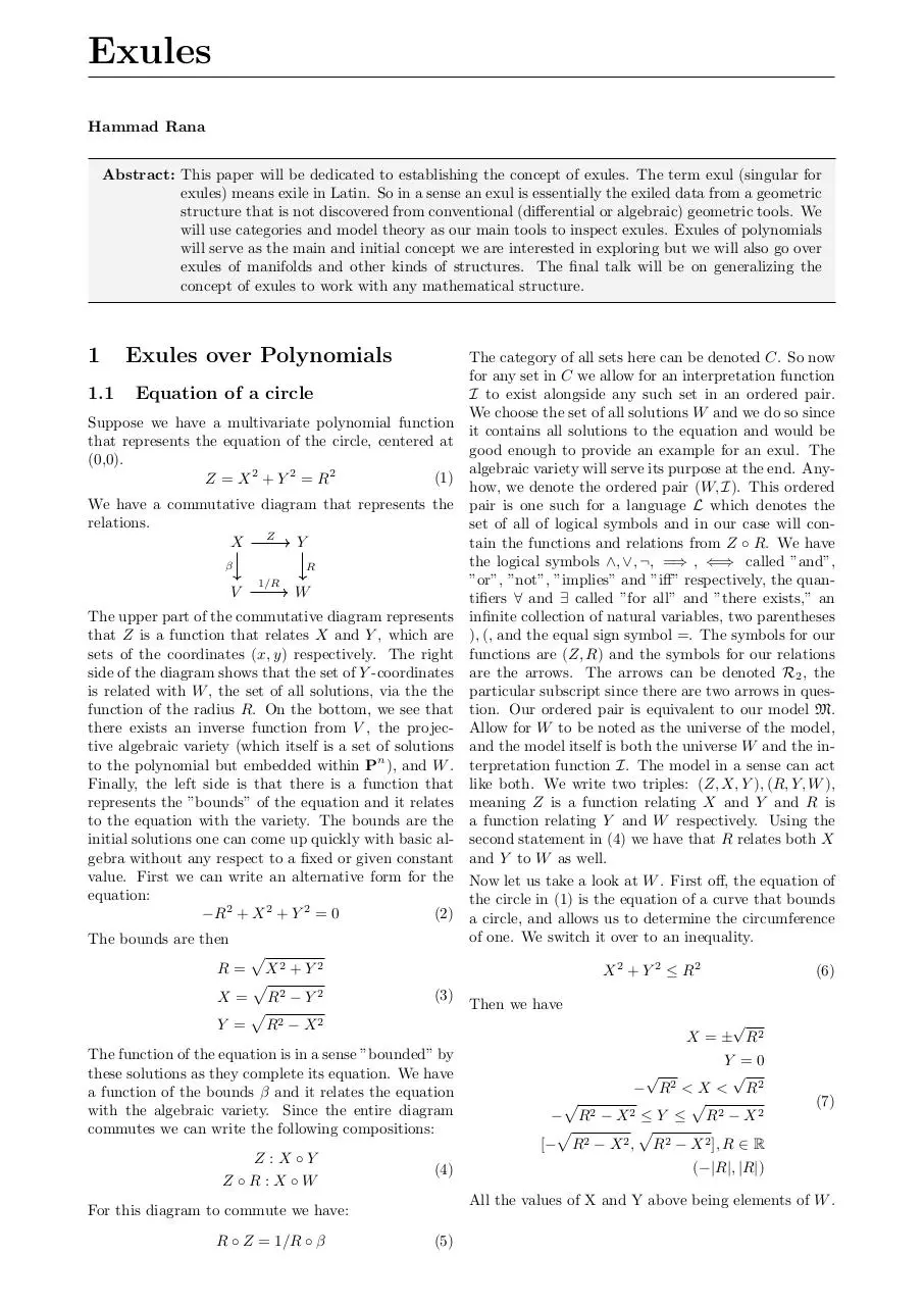
We have a commutative diagram that represents the
relations.
X Z Y
β

V

R
1/R

W

The category of all sets here can be denoted C. So now
for any set in C we allow for an interpretation function
I to exist alongside any such set in an ordered pair.
We choose the set of all solutions W and we do so since
it contains all solutions to the equation and would be
good enough to provide an example for an exul. The
algebraic variety will serve its purpose at the end. Anyhow, we denote the ordered pair (W, I). This ordered
pair is one such for a language L which denotes the
set of all of logical symbols and in our case will contain the functions and relations from Z ◦ R. We have
the logical symbols ∧, ∨, ¬, =⇒ , ⇐⇒ called ”and”,
”or”, ”not”, ”implies” and ”iff” respectively, the quantifiers ∀ and ∃ called ”for all” and ”there exists,” an
infinite collection of natural variables, two parentheses
), (, and the equal sign symbol =. The symbols for our
functions are (Z, R) and the symbols for our relations
are the arrows. The arrows can be denoted R2 , the
particular subscript since there are two arrows in question. Our ordered pair is equivalent to our model M.
Allow for W to be noted as the universe of the model,
and the model itself is both the universe W and the interpretation function I. The model in a sense can act
like both. We write two triples: (Z, X, Y ), (R, Y, W ),
meaning Z is a function relating X and Y and R is
a function relating Y and W respectively. Using the
second statement in (4) we have that R relates both X
and Y to W as well.

The upper part of the commutative diagram represents
that Z is a function that relates X and Y , which are
sets of the coordinates (x, y) respectively. The right
side of the diagram shows that the set of Y -coordinates
is related with W , the set of all solutions, via the the
function of the radius R. On the bottom, we see that
there exists an inverse function from V , the projective algebraic variety (which itself is a set of solutions
to the polynomial but embedded within Pn ), and W .
Finally, the left side is that there is a function that
represents the ”bounds” of the equation and it relates
to the equation with the variety. The bounds are the
initial solutions one can come up quickly with basic algebra without any respect to a fixed or given constant
value. First we can write an alternative form for the Now let us take a look at W . First off, the equation of
equation:
the circle in (1) is the equation of a curve that bounds
−R2 + X 2 + Y 2 = 0
(2) a circle, and allows us to determine the circumference
of one. We switch it over to an inequality.
The bounds are then
p
R = X2 + Y 2
(6)
X 2 + Y 2 ≤ R2
p
2
2
(3)
X = R −Y
Then we have
p
√
Y = R2 − X 2
X = ± R2
The function of the equation is in a sense ”bounded” by
Y =0
these solutions as they complete its equation. We have
√
√
− R2 < X < R2
a function of the bounds β and it relates the equation
p
p
(7)
with the algebraic variety. Since the entire diagram
− R2 − X 2 ≤ Y ≤ R2 − X 2
p
p
commutes we can write the following compositions:
[− R2 − X 2 , R2 − X 2 ], R ∈ R
Z :X ◦Y
(−|R|, |R|)
(4)
Z ◦R:X ◦W
All the values of X and Y above being elements of W .
For this diagram to commute we have:
R ◦ Z = 1/R ◦ β

(5)