ProjectReport (PDF)

Spam Email Classifier
With the addition of POS tags

CSE 390
By: Erik Emmanuel
Brian Lin
Jianneng (Jack) Wu

05/04/2017
Professor Niranjan Balasubramanian
TA: Noah Weber

Spam Email Classifier
Natural Language Processing has allowed us to be able to allow
computers to extract the meaning behind our language. This has given us
the proper tools to be able to build the spam email classifier. The classifier
is designed to filter emails by removing the emails that were reported to be
sent by another computer. We choose this topic for our project because we
were building something that in turn could help save people a lot of time.
Although the limits of our project are extended to a limit dataset, we can
understand the workings of how filtering can be done. The project will
consist of 3 parts. In part 1 we build the training data needed to make the
classifier. Part 2 will then be to build the Naive Bayes algorithm and test it
on a new set of data. Afterwards we will also measure the performance of
the classifier measuring F-1 score, recall and precision. The last part will
then to be implement part of speech tagging to further improve the
performance of the classifier.

Probability generation for training dataset (Part 1: Erik)
Vocab set generation:
For the data extraction, We used the data we acquired from the Enron dataset.
From the dataset we used the preprocessed data which was already categorized as
either spam or not spam (ham). In the training set there was 5975 unique emails, and of
those there was 1:3 ratio of spam to ham emails. For the probability generation aspect
of the project we made a python script that goes through a folder, opens each folder
and and for each line in the email tokenize the word. Make counts of each word and
how many times they had occurred in each of the classes (spam or ham). For every
new word that was observed it was added to the vocab array. Since the dataset was
large, I omitted tokens from emails that were not words; ie. “12” was not considered as it
is a number while “NBA’16” would be an example of an alphanumeric token that was
considered part of the vocab. I also omitted words from the vocab that occurred less
than 2 times.Once the dataset was finalized, I had to attach probabilities that the word
could lead to the document being classified as a spam or ham email.

Probability Extraction:
Once the vocab array was finalized, now we had to go through each object in the
list and calculate the probability that word either lead to a spam or ham. To determine
the P(spam|word) and P(ham|word).
P (wi |spam) =

#(wi occurred in spam)
#(wi occurred in total)

P (wi |ham) =

#(wi occurred in ham)
#(wi occurred in total)

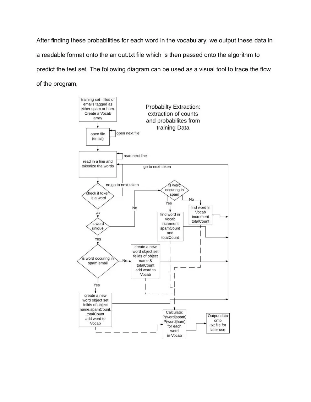
After finding these probabilities for each word in the vocabulary, we output these data in
a readable format onto the an out.txt file which is then passed onto the algorithm to
predict the test set. The following diagram can be used as a visual tool to trace the flow
of the program.

Implementation of Naive Bayes Algorithm (Part 2: Brian)
At this point we had our training data from the training emails in the form of
out.txt. Now our task was to create a process in which we can process new unknown
emails and determine from the training data whether or not the email is valid or spam.
This is where the Naive Bayes Algorithm comes into play.
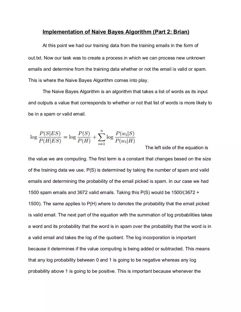
The Naive Bayes Algorithm is an algorithm that takes a list of words as its input
and outputs a value that corresponds to whether or not that list of words is more likely to
be in a spam or valid email.

The left side of the equation is
the value we are computing. The first term is a constant that changes based on the size
of the training data we use. P(S) is determined by taking the number of spam and valid
emails and determining the probability of the email picked is spam. In our case we had
1500 spam emails and 3672 valid emails. Taking this P(S) would be 1500/(3672 +
1500). The same applies to P(H) where to denotes the probability that the email picked
is valid email. The next part of the equation with the summation of log probabilities takes
a word and its probability that the word is in spam over the probability that the word is in
a valid email and takes the log of the quotient. The log incorporation is important
because it determines if the value computing is being added or subtracted. This means
that any log probability between 0 and 1 is going to be negative whereas any log
probability above 1 is going to be positive. This is important because whenever the

probability of the word being in spam is greater than it being in a valid email then the
value of log((w|S)/(w|H)) is going to be positive. The only way that a email is classified
as spam is when the final value of the right side is above 0.
We tested this algorithm on the test set called enron2 which contained 4361 valid
emails and 1496 spam emails. Running through the emails with the implemented
algorithm gave us the results:
Spam: Recall = 0.4525
Ham: Recall = 0.8167

Precision = 0.9713 F-1 = 0.6174
Precision = 0.7737 F-1 = 0.7947

The precision in the classifier for spam emails was amazing, almost every email that the
classifier predicted as spam came out to actually be spam. However the recall of spam
emails was very poor. Less than half of the emails that were spam were detected by the
classifier. I believe the reason behind this is the training data. Because of the fact that
the number of spam emails was much less than the number of the valid emails in the
training set, this causes the words in the training set to have more frequent words where
the probability of the word being in a valid email is greater than the probability of the
word in a spam email. This affects the equation, more precisely

. The

fraction will then be a value between 0 and 1 and any log of that value will produce a
negative value. Adding a negative to the equation will skew the equation to return that
the email is valid

and for that the recall is imperfect. This could be fixed if

we were to have

more data for training where the ratio of spam and valid

emails were closer to 1.

Figure 2.1 Flowchart of Algorithm
Implementation

POS Tagging and the Naive Bayes Algorithm (Part 3: Jack)
Training:
Using the Enron1 data from the Enron dataset​1​, I tagged the data using a POS tagger​2
from Stanford. I chose to use this over using the one that we made for two reasons; It’s
much more accurate (97% Precision), and it’s much for efficient. With so much training
data, efficiently tagging the data is quite important. Passing the paths of the data to
pos_tagger.java ​, outputs the results a directory named “enron_tagged”. Then using
train_tagger.py​, and the path to the tagged ham/spam folders, we can calculate their
emissions probabilities: P (T |W ). This is outputted as “emissions_ham.txt” and
“emissions_spam.txt”.

Modifying the algorithm:
Given the existing algorithm from a research paper​3​ by Tianhao Sun, we were able to
implement the existing algorithm as follows:

P (S|E)
log P (H|E)

=

P (S)
log P (H)

n

P (w |S)

+ ∑ log P (w i|H)
i=1

i

Where if the result is greater than zero, then we classify if as spam. For the POS
adjustment I will be integrating interpolation into the function for one main reason: I
generally understand the concept and feel this is a good and simple probability
distribution for combining two “features”. I will be modifying the equation as follows:

P (wi |S, ti ) =

λ1 P (wi ⋂S)+λ2 P (wi |S,ti )
and​
P (S)

P (wi |H, ti ) =

λ1 P (wi ⋂H)+λ2 P (wi |H,ti )
P (H)

Where λ​1​ and λ​2​ are weights assigned to each feature. For our specific case we used
λ​1​=0.9 and λ​2​=0.1 because these weights provided generally the best results. The final
equation for determining if the email is classified as a spam is then as follows:

P (S|E)
log P (H|E)

=

P (S)
log P (H)

n

P (w |S,t )

+ ∑ log P (w i|H,ti )
i=1

i

i

*** At this point is where I’m not sure if I normalized correctly as there are little to no
research papers detailing the addition of POS tags with respect to the Naive Bayes
Algorithm.

Testing:
To test the algorithm, I used the stanford tagger to tag the next set of the enron dataset
(enron2). I then modified the original code from Brian Lin (​WordProb.py​) to adjust for my
changed input data along with additional emissions data, and created the code
WordProbPOS.py .​ After optimizing the code, I ran the algorithm a few times to test sets
of weights that would be appropriate and settled on 0.9 and 0.1 respectively.

Results and Concerns With the POS Method:
From the results (specified below), we can see that with the addition of the POS tags,
we have decreased the precision of the algorithm by around 5% with respect to the
original algorithm, but have increased the recall by an astounding 45%. This is where
my concerns lie: I’m not 100% certain that I normalized the probabilities correctly, and