Predictive Understanding of Critical Phenomena

On Predictive Understanding of Extreme Events: Statistical Physics Approach; Prediction Algorithms; Applications to Disaster Preparedness Vladimir Keilis-Borok1,2,3, Alexandre Soloviev2,3, Andrei Gabrielov4 1 Inst. of Geophysics and Planetary Physics and Dept. of Earth and Space Sciences, University of California, Los Angeles, USA, email: vkb@ess.ucla.edu. 2 Int. Inst. of Earthquake Prediction Theory and Mathematical Geophysics, Russian Ac. Sci., Moscow, Russia, email: soloviev@mitp.ru. 3 The Abdus Salam Int. Centre for Theoretical Physics, Trieste, Italy. 4 Departments of Mathematics and Earth & Atmospheric Sciences, Purdue University, USA, email: agabriel@math.purdue.edu. Abstract We describe a uniform approach to predicting different extreme events, also known as critical phenomena, disasters, or crises. Following types of such events are considered: strong earthquakes; economic recessions (their onset and termination); surges of unemployment; surges of crime; and electoral changes of governing party. A uniform approach is possible due to the common feature of these events: each of them is generated by a certain hierarchical dissipative complex system. After a coarsegraining, such systems exhibit regular behavior patterns; we look among them for the “premonitory patterns”, that signal approach of an extreme event. These patterns might be either “perpetrators” contributing to the triggering the extreme event, or “witnesses” merely signaling that the system has become unstable, ripe for such an event. Methodology. Prediction algorithms have been developed by “pattern recognition of infrequent events” – the methodology developed by the school of I. Gelfand; it integrates exploratory data analysis with theoretical and numerical modeling. Major results -- Prediction algorithms are developed for the extreme events of each type considered. As required in complexity studies these algorithms are robust and self-adjusting to the scale of the system, level of its background activity, magnitude of prediction targets etc. Accuracy of prediction is defined by the rate of false alarms, rate of failures to predict, and total time-space occupied by the alarms. The algorithms allow choosing the tradeoff between these characteristics. -- New understanding of the origin of the extreme events considered is also developed. -- Linking prediction with disaster preparedness. We introduce methodology assisting disaster management in choosing optimal set of disaster preparedness measures undertaken in response to a prediction. Methodology is based on the optimal control theory. So far it was applied only to earthquakes. Importantly, predictions with their currently realistic (limited) accuracy do allow preventing a considerable part of the damage by a hierarchy of preparedness measures. Accuracy of prediction should be known, but not necessarily high. 1  I. Introduction Prediction problem. Targets of prediction are individual extreme events that are rare but make big impact. 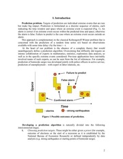Prediction is formulated as a discrete sequence of alarms, each indicating the time window and space where an extreme event is expected (Fig. 1). An alarm is correct if an extreme event occurs within the predicted time and space; otherwise the alarm is false. Failure to predict is the case where an extreme event occurs outside an alarm. This approach is complementary to the classical Kolmogoroff-Wiener problem that is concerned with the prediction of a random time series x(t) based on observations available with some time delay τ by the time t – τ. At the heart of our problem is the absence of a complete theory that would unambiguously define a prediction algorithm. Overcoming that difficulty did require an intense collaboration of experts in mathematics, statistics, exploratory data analysis, as well as in the specific extreme events considered. Previous applications have inevitably involved teams of such experts, as can be seen from the list of references. For example, prediction of homicide surges was developed jointly with police officers in active service; prediction of unemployment – with expert in labor relations, etc. Figure 1 Possible outcomes of prediction. Developing a prediction algorithm is naturally divided into the following interconnected stages. 1. Choosing prediction targets. These might be either given a priori (for example, outcome of elections or the start of a recession as it is established by the National Bureau of Economic Research) or defined independently by data analysis (e.g. strong earthquakes or starting points of homicide surge). 2  2. 3. 4. Choosing the background fields where we hope to detect precursors. For example, prediction of strong earthquakes was based on seismicity patterns in lower magnitude range; prediction of recessions was based on six leading economic indicators. Any potentially relevant field can be considered. Formulation of a hypothetical prediction algorithm. That is done by the pattern recognition of rare events – the methodology developed by the school of I. Gelfand for studying rare events of highly complex origin (e.g., Bongard, 1970; Gelfand et al., 1976; Keilis-Borok and Lichtman, 1993; Press and Allen, 1995; Keilis-Borok et al., 2000, 2003, 2005, ). Validation of prediction algorithm by prediction in advance. Prediction quality is characterized by three scores: rate of false alarms, rate of failures-to-predict, and total space-time occupied by alarms (as percentage of total spacetime considered). These characteristics are important to decision-makers choosing what, if any, preparedness measures to undertake in response to an alarm. Predictability. Extreme events targeted by our predictions have a consequential common feature: they are generated by complex (chaotic) systems such as seismically active lithosphere, society, or economy. Complex systems are often regarded as unpredictable in principle. Actually, after a coarse-graining, on a not-too-detailed scale, such systems do exhibit the regular behavior patterns. Among them are premonitory patterns that emerge more frequently as an extreme event approaches. Thus extreme events become predictable up to a limit. Premonitory patterns might be either “perpetrators” contributing to the triggering the extreme event, or “witnesses” merely signaling that the system has become unstable, ripe for such an event. An example of a witness are proverbial straws of the wind preceding a hurricane. 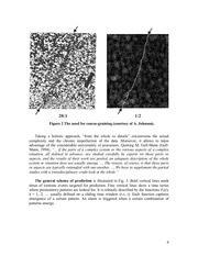The need for coarse-graining is illustrated in Fig. 2: a crack is visible only on a less detailed scale. “It is not possible to understand chaotic system by breaking it apart” (Crutchfield et al., 1986). 3  20:1 1:2 Figure 2 The need for coarse-graining (courtesy of A. Johnson). Taking a holistic approach, “from the whole to details” circumvents the actual complexity and the chronic imperfection of the data. Moreover, it allows to takes advantage of the considerable universality of precursors. Quoting M. Gell-Mann (GellMann, 1994), “... if the parts of a complex system or the various aspects of a complex situation, all defined in advance, are studied carefully by experts on those parts or aspects, and the results of their work are pooled, an adequate description of the whole system or situation does not usually emerge. … The reason, of course, is that these parts or aspects are typically entangled with one another. 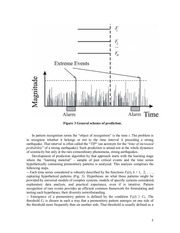… We have to supplement the partial studies with a transdisciplinary crude look at the whole.” The general scheme of prediction is illustrated in Fig. 3. Bold vertical lines mark times of extreme events targeted for prediction. Fine vertical lines show a time series where premonitory patterns are looked for. It is robustly described by the functions Fk(t), k = 1, 2, … usually defined on a sliding time window (t-s, t). Each function captures emergence of a certain pattern. An alarm is triggered when a certain combination of patterns emerge. 4  Figure 3 General scheme of prediction. In pattern recognition terms the “object of recognition” is the time t. The problem is to recognize whether it belongs or not to the time interval ∆ preceding a strong earthquake. That interval is often called the “TIP“ (an acronym for the “time of increased probability” of a strong earthquake). Such prediction is aimed not at the whole dynamics of seismicity but only at the rare extraordinary phenomena, strong earthquakes. Development of prediction algorithm by that approach starts with the learning stage where the ”learning material” – sample of past critical events and the time series hypothetically containing premonitory patterns is analyzed. This analysis comprises the following steps. -- Each time series considered is robustly described by the functions Fk(t), k = 1, 2, . . . , capturing hypothetical patterns (Fig. 3). Hypotheses on what these patterns might be provided by universal models of complex systems, models of specific systems considered, exploratory data analysis, and practical experience, even if is intuitive. Pattern recognition of rare events provides an efficient common framework for formulating and testing such hypotheses, their diversity notwithstanding. -- Emergence of a premonitory pattern is defined by the condition Fk(t) ≥ Ck. The threshold Ck is chosen in such a way that a premonitory pattern emerges on one side of the threshold more frequently then on another side. That threshold is usually defined as a 5  certain percentile of the functional Fk(t). Thus the time series Fk(t) is presented on the lowest – binary – level of resolution. -- An alarm is triggered at a time ta, when certain combination of patterns occurs; this combination is determined by application of the pattern recognition procedure. Detailed description of pattern recognition methodology can be found in Bongard (1970), Gelfand et al. (1976), Keilis-Borok and Lichtman (1993), Keilis-Borok and Soloviev (2003). Four paradigms on premonitory patterns have been established (Keilis-Borok, 2002; Keilis-Borok and Soloviev, 2003) provide a guidance for the choice of functions Fk(t). Paradigm 1: Basic types of premonitory patterns. These are illustrated in Fig. 4. As an extreme event draws near, the background activity becomes more intense and clustered in space–time, while the radius of correlation in space increases and size distribution (scaling relation) shifts in favor of relatively stronger events. Paradigm 2: Long-range correlations. Generation of an extreme event is not localized in its vicinity. For example, according to Press and Allen (1995), the Parkfield, California earthquake with the characteristic source dimension 10 km “... is not likely to occur until activity picks up in the Great Basin or the Gulf of California”, about 800 km away. Numerous evidences for that paradigm are described also by Mogi (1968), Aki (1996), Press and Briggs (1975), Keilis-Borok and Press (1980), Ma et al. (1990), Romanowicz (1993) etc. In the case of seismicity these correlations may be explained by several mechanisms that range from micro-fluctuations of large scale tectonic movements to impact of migrating fluids (e.g., Barenblatt et al., 1983; Barenblatt, 1993; Press and Allen, 1995; Sornette and Sammis, 1995; Aki, 1996; Bowman et al., 1998; Pollitz et al., 1998; Turcotte et al., 2000). An example of the long-range correlation in a socioeconomic system is surge of ethnic violence in a French suburb, preceded by a rise in ethnic delinquency countrywide (Bui Trong, 2003). Paradigm 3: Similarity. Quantitative definition of prediction algorithms is selfadjusting to regional conditions. For example, earthquake prediction algorithms developed for seismicity of California retain their predictive power for other regions worldwide, for starquakes, and, at the other end of the spectrum, for fracturing in engineering constructions and laboratory samples (e.g., Keilis-Borok et al., 1980; Aki, 1996; Rotwain et al., 1997; Keilis-Borok and Shebalin, 1999; Kossobokov et al., 2000; Kossobokov and Shebalin, 2003; Keilis-Borok and Soloviev, 2003). The energy of a target event in these applications ranges from ergs (micro-fracture) to 1026 ergs (major earthquake), and even to 1041 ergs (starquake). Another example is an algorithm for predicting the surge of unemployment, applicable “as is” to the United States, France, Germany, and Italy (Keilis-Borok et al., 2005). 6  Safe stage Pre-disaster stage Figure 4 Four types of premonitory patterns. Paradigm 4. Dual nature of premonitory patterns. The premonitory patterns shown in Fig. 4 are “universal”, common for hierarchical complex systems of different origin. They can be reproduced in the models of dynamical clustering (Gabrielov et al., 2008), branching diffusion (Gabrielov et al., 2007), percolation (Zaliapin et al., 2005, 2006), direct, inverse, and colliding cascades (Allègre et al., 1982; Narkunskaya and Shnirman, 1994; Shnirman and Blanter, 1999, 2003; Gabrielov et al., 2000; Zaliapin et al., 2003; Yakovlev et al., 2005), as well as in certain system-specific models (e.g., Soloviev and Ismail-Zadeh, 2003; Sornette, 2004). Coping with risk of data fitting. Being not defined unambiguously by an existing theory, our prediction algorithms inevitably include some adjustable elements, from selecting the data used for prediction to the values of numerical parameters. These elements are adjusted retrospectively by “predicting” past extreme events. Such data-fitting might be self-deceptive: as J. von Neumann put it “with four exponents I can fit an elephant”. Hence, the following tests are made. - Sensitivity analysis: predictions should be not too sensitive to variations in adjustable elements. - Out of sample analysis: application of an algorithm to past data that has not been used in the algorithm's development. The test is considered successful if the accuracy of prediction does not drop too far. - Finally - Prediction in advance. 7  II. Predicting individual extreme events EARTHQUAKES Relatively better tested so far are the algorithms based on premonitory seismicity patterns (Keilis-Borok, 1990, 2002; Keilis-Borok and Shebalin, 1999; Kossobokov and Shebalin, 2003; Keilis-Borok and Soloviev, 2003; Peresan et al., 2005). The predictions are filed in advance on the following websites: http://www.mitp.ru/predictions.html; http://users.ictp.it/www_users/sand/index_files/DevelopmentofPrediction.html; and http://rtptest.org/. Access to yet unexpired alarms on these websites is limited to about 200 scientists and professional experts worldwide. This is done in compliance to the UNESCO guidelines, since public release of prediction might trigger disruptive anxiety of population and profiteering. Predictions are made available for general public after a strong earthquake occurs or alarm expires, whichever comes first. Figure 5 Alarms capturing the Sumatra earthquake, 4 June 2000. Yellow - area of alarm by M8, put on record in July 1996, to expire on July 1, 2001. Red - reduction of the alarm area by MSc, put on record in January 1998. White circles epicenters of Sumatra earthquake and its first-month aftershocks. M8 and MSc algorithms (Kossobokov and Shebalin, 2003). Algorithm M8 provides intermediate-term predictions. Characteristic duration of an alarm is about 5 years. That algorithm was first developed for predicting the largest earthquakes (M ≥ 8) worldwide. The algorithm MSc (“Mendocino Scenario”) provides a second approximation to M8, strongly reducing the alarm area. Figure 5 shows an example of prediction by both algorithms. 8  Scoring. Thus far, the algorithms have had most success in predicting future earthquakes in the magnitude range 8–8.5 (Table 1). Statistical significance of predictions exceeds 99%. Table 1. Scoring of M8 and M8 & MSc predictions, 1992-2010 Algorithm Total number of target earthquakes Number of predicted earthquakes Space-time volume of alarm M8 17 12 29% M8 & MSc 17 8 15% “Second Strong Earthquake” (SSE) algorithm (Levshina and Vorobieva, 1992; Vorobieva, 1999, 2009). That algorithm is applied when a strong earthquake of a certain magnitude M has occurred. The algorithm predicts whether a second strong earthquake with magnitude (M – 1) or more will occur within 18 months of the first one, within a distance R depending on magnitude M; R = 0.03x100.5M km that is one and a half of the aftershock area linear size for an earthquake with magnitude M (Tsuboi, 1956). Figure 6 shows an example of SSE prediction made after the Landers earthquake, June 28, 1992, M = 7.6. Prediction was released in EOS, October 1992, with alarm ending on December 28, 1993. A second strong earthquake M ≥ 6.6 was predicted to occur within the yellow circle. On January 17, 1994, 20 days after the alarm expired, the Northridge earthquake (M = 6.8) did occur and resulted in 57 deaths, more than 5,000 injuries, and more than $20 billion in property damage. For the sake of rigorous scoring, this earthquake was counted as not predicted. On the practical side, escalation of preparedness measures in response to this prediction would be fully justified. Scoring. Since 1989 the SSE algorithm is being tested in ten regions worldwide (Vorobieva, 1999, 2009), with the magnitude of the first events ranging from 5 or above in the Dead Sea Rift region, to 7 or more in the Balkans. In total, 31 first events have been considered. Eight of them were followed by a second strong earthquake within 18 months; 6 have been predicted and 2 missed. For the remaining 23 single events, 19 correct predictions and 4 false alarms have been made. Statistical significance of these predictions is above 99%. 9  Figure 6 Prediction of Northridge, California earthquake by SSE algorithm. “Reverse Tracing of Precursors” (RTP) algorithm (Shebalin et al., 2004, 2006; Keilis-Borok et al., 2004a). The algorithm is aimed at predictions about 9 months in advance, much shorter than by the M8 and SSE algorithms. This algorithm, as its name suggests, traces precursors in the reverse order of their formation. First it identifies “candidates” for short-term precursors. These are long, quickly formed chains of earthquakes in the background seismicity. Such chains reflect an increase in the earthquake correlation range (Fig. 7): each is examined to determine whether there had been any preceding intermediate-term precursors in its vicinity within the previous five years. If so, the chain triggers an alarm. This approach has natural applications to a variety of extreme events. Scoring. Since 2003, the RTP algorithm has been tested by predicting future earthquakes in five regions of the world (California and adjacent regions; Central and Northern Italy with adjacent regions; Eastern Mediterranean; Northern Pacific, Japan and adjacent regions). So far five out of seven target earthquakes have been predicted (captured by alarms) and two missed. Out of 19 alarms, five were correct and fourteen false, two of the latter being near misses occurring close to alarm areas. The data are still insufficient for rigorous estimation of statistical significance. 10  Figure 7 RTP Prediction of the 2006-2007 Simushir earthquakes in Kuril Islands Red contour - area of alarm issued on October 2006 for 9 months. This was confirmed by the earthquake of November 15, 2006, M=8.3. Stars – predicted earthquakes. US PRESIDENTIAL ELECTIONS. Tradition regards American elections as a trial by battle, where the goal of the competitors is to attract a maximum number of voting blocks with minimal alienation of other blocks. The outcome depends strongly on manipulation of public opinion and lastminute sensations. Accordingly, that tradition ascribes the victory of George H.W. Bush in 1988 to three brilliant campaigners: speechwriter Peggy Noonan improved his image overnight by New Orleans speech; two hardball politicians staged mass-media exposure of failure of M. Dukakis as a Governor of Massachusetts. Furthermore M. Dukakis fired a good campaigner. As a result he lost elections, which were in his grasp (he led by 17% in opinion polls). This notion tells us that a huge mass of voters can reverse its opinion through the influence of three campaigners and the loss of one, in a “for-want-of-a-nail-the-war-waslost” fashion. In other words, it portrays Jane/Joe Voter as an excitable simpleton, manipulated by commercials, reversing its vote for transient reasons, irrelevant to the essence of the electoral dilemma. American elections deserve a more dignified explanation. An alternative view, contrasting with that described above, was developed by holistic approach, fitting understanding electorate as a hierarchical complex system (Keilis-Borok and Lichtman, 1981). Here, election outcome depends on coarse-grained socio-economic and political factors of the common-sense type. These factors were given a robust definition as yes/no questionnaire responses. The actual electoral dilemma is found to be whether the incumbent party will win or lose rather than whether the Republicans or Democrats will win. 11  Prediction algorithm (Lichtman and Keilis-Borok, 1989; Keilis-Borok and Lichtman, 1993; Lichtman, 1996, 2000, 2005).is defined in Table 2. It was developed by pattern recognition analysis of the data on the 31 past elections, 1860-1980; that covers the period between victories of A. Lincoln and R. Reagan. The Keys are stated to favor the re-election of the incumbent party. When five or fewer are false, the incumbent party wins. When six or more are false, the other party wins. Table 2. Keys used for prediction of the outcome of the Presidential elections in the U.S. Relevance KEY 1 KEY 2 KEY 3 KEY 4 KEY 5 KEY 6 KEY 7 KEY 8 KEY 9 KEY 10 KEY 11 KEY 12 KEY 13 Statement to favor the re-election of the incumbent party Party Mandate After the midterm elections, the incumbent party holds more seats in the U.S. House of Representatives than it did after the previous midterm elections. Contest There is no serious contest for the incumbent-party nomination. Incumbency The incumbent-party candidate is the sitting president. Third party There is no significant third party or independent campaign. Short-term The economy is not in recession during the election economy campaign. Long-term Real per-capita economic growth during the term equals economy or exceeds mean growth during the previous two terms. Policy change The incumbent administration effects major changes in national policy. Social unrest There is no sustained social unrest during the term. Scandal The administration is untainted by major scandal. Foreign/military The administration suffers no major failure in foreign or failure military affairs. Foreign/military The administration achieves a major success in foreign or success military affairs. Incumbent The incumbent-party candidate is charismatic or a charisma national hero. Challenger The challenging-party candidate is not charismatic or a charisma national hero. Results of retrospective analysis and advance predictions made by A. Lichtman since 1984 are shown in Table 3. All seven presidential elections have been predicted correctly. That includes Al Gore’s victory by popular vote which was reversed by electorate; this happened 3 times through the whole history. Timing and source of the predictions are listed in Table 4. 12  Table 3. Prediction of US presidential elections Red - incumbent won; blue – challenger won; * years when popular vote was reversed by electoral vote. Predictions (published months in advance) 2000* 1984 1988 2004 1996 1992 2008 Retrospective analysis 1964 1980 1928 1976 1916 1968 1908 1952 1944 1900 1972 1932 1956 1940 1872 1924 1948 1912 1884 1920 1960 1904 1936 1868 1864 1880 1888* 1892 1860 1896 1876* 0 1 2 3 4 5 6 7 8 9 Number of keys in favor of a challenger party Table 4. Timing and source of predictions Election Date of prediction Source 1984 April 1982 “How to Bet in ’84,” Washingtonian Magazine, April 1982 1988 May 1988 “How to Bet in November,” Washingtonian Magazine, May 1988 1992 September 1992 “The Keys to the White House,” Montgomery Journal, September 14, 1992 1996 October 1996 “Who Will Be the Next President?” Social Education, October 1996 2000 November 1999 “The Keys to Election 2000” Social Education, November/December 1999. 2004 April 2003 “The Keys to the White House,” Montgomery Gazette, Apr. 25, 2003 2008 February 2006 “Forecast for 2008,” Foresight, Feb. 2006, As of now, only 4 Keys in Table 2, are false, so the algorithm predicts victory for Barak Obama in November 2012 (Lichtman, 2010). 13  What have we understood about the elections? Uniformity of prediction rules transcends the diversities of situations prevailing in individual elections. Accordingly, the same pattern of the choice of president has prevailed since 1860, i.e., since election of A. Lincoln, throughout all the overwhelming changes of these 140 years. And in particular, note that the electorate of 1860 did not include the groups making up 75% of the present electorate: no women, blacks, or most of the citizens of Latin American, South European, East European and Jewish descent (Lichtman, 2000). In a nutshell, we have found that the outcome of a presidential election is determined by collective estimation of performance of incumbent administration over the previous four years. SURGE OF UNEMPLOYMENT RATE Here we describe uniform prediction of the sharp and long-term rise in unemployment in France, Germany, Italy, and the U.S. (Keilis-Borok et al., 2005) – we term this FAU, which is an acronym for “Fast Acceleration of Unemployment”. The data comprise macroeconomic indicators of national economy. In stability tests a variety of other indicators were also analyzed. Figure 8 shows retrospective alarms. Exactly the same self-adjusting algorithm was applied to all four countries. France Germany Italy USA 60 65 70 75 80 85 90 95 Figure 8 FAUs and alarms in the four countries Vertical lines – prediction targets (FAUs). Red – correct alarms, purple - alarms triggered within the periods of unemployment surge, blue – false alarms. The 1968 alarm is scored as false since it expired one month before FAU. 14  Prediction-in-advance has been in progress since 1999, so far only for the U.S. Two recent episodes of FAU have been predicted correctly, without failures to predict or false alarms (Fig. 9). 10 Unemployment rate, % 9 8 7 6 5 4 3 2000 2001 2002 2003 2004 2005 2006 2007 2008 2009 2010 2011 Time Figure 9 Made-in-advance predictions of FAUs. The thin blue curve shows the monthly unemployment rate in USA, according to the data of the Bureau of Labor Statistics, U.S. Department of Labor (http://data.bls.gov). The bold curve shows this rate with seasonal variation smoothed out. Vertical red lines prediction targets (FAUs); gray bar – period of unemployment growth; pink bars – periods of alarms. US ECONOMIC RECESSIONS Prediction targets are the peaks and troughs of economic activity, i.e. the first and last months of each recession as identified by the National Bureau of Economic Research (NBER). The data used in the prediction algorithm comprise six monthly leading economic indicators, reflecting interest rates, industrial production, inventories, and job market (Keilis-Borok et al., 2000, 2008). Retrospective alarms and recessions are shown together in Fig. 10. We see that five recessions occurring between 1961 and 2000 were preceded by an alarm. The sixth recession started in April 2001, one month before the corresponding alarm. In practice, this is not a failure-to-predict, since recessions are usually declared by NBER much later than they begin. The duration of each alarm was 1 to 14 months. Total duration of all 15  alarms was 38 months, or 13.6% of the time interval considered. There was only one false alarm in 2003. Advance prediction Prediction of recessions 1960 1965 1970 1975 1980 1985 1990 1995 2000 2005 2010 1995 2000 2005 2010 Prediction of recovery from recessions 1960 1965 1970 - Recession 1975 1980 1985 1990 - Alarm Figure 10 Prediction of economic recessions in the U.S. Accordingly to the NBER announcement issued in December 2008 the last recession in the U.S. began in January 2008. Our algorithm gave an alarm started in May 2008 that is four months after the recession start but seven months before the NBER announcement. The same six macroeconomic indicators have been used to develop an algorithm for prediction of the recovery from a recession (Keilis-Borok et al., 2008). The algorithm declares alarms within 6 months before the end of each American recession since 1960 and at no other time during these recessions (Fig. 10). This study is a natural continuation of the previous one, aimed at predicting the start of a recession. Comparing these cases we find that precursory trends of financial indicators are opposite during transition to a recession and recovery from it. To the contrary, precursory trends of economic indicators happen to have the same direction (upward or downward) but are steeper during recovery. The algorithm declares an alarm starting in November 2008 for the end of the last recession. HOMICIDES SURGES Prediction target is the start of a sharp and lasting rise (“a surge”) of the homicide rate in an American megacity – Los Angeles. Data comprise by monthly rates of 11 types of low-level crimes: burglaries, assaults, and robberies. Statistics of these types of crime in Los Angeles over the period 19752002 has been analyzed to find an algorithm for predicting such a surge of the homicide rate (Keilis-Borok et al., 2003). Premonitory patterns include: first - escalation of burglaries and assaults, but not of robberies; closer to a homicide surge, robberies also escalate. It has been found in retrospective analysis that this algorithm is applicable through all the years considered despite substantial changes both in socio-economic conditions and 16  in the counting of crimes. Alarms and homicide surges are plotted together in Fig. 11. In total, alarms occupy 15% of the time considered. Moreover, the algorithm gives satisfactory results for the prediction of homicide surges in New York City as well. Figure 11 Prediction of homicide surges in Los Angeles. III. “Barometer” signaling approach of a disaster This is the software assisting the governance in foreseeing disasters. It detects symptoms of a disaster’s approach. Obvious examples are low atmospheric pressure measured by the usual barometers and high body temperature in medicine. The input to the software comprises the indicators relevant to disasters considered. The output signals whether or not such a disaster is approaching. This information is less specific but more robust than prediction; it gives a decision-maker important quantitative characteristics of the current threat. Below we demonstrate a barometer based on premonitory transformation of scaling relation (see lower panel in Fig. 4). To capture that transformation we compare the scaling of background activity of the system in the time periods of three kinds: D preceding an extreme event; X – following it; N - others (Fig. 12). Scaling is defined as P(m) = Ptot(m)/Ňtot, where Ptot is the number of events of the size ≥ m, Ňtot is the total number of events (obviously, P(m) is equivalent to statistical distribution function). 17  Figure 12 Division of time into intervals D, N, and X. Figures 13-15 show premonitory changes in scaling P(m) before strong earthquakes, socio-economic crises, and surges of terrorism. Figure 16 shows the same effect for two models of complex systems: branching diffusion and dynamic clustering (Gabrielov et al., 2007, 2008). Figure 13 Premonitory transformation of scaling - earthquakes Prediction targets - main shocks with magnitude M ≥ 8 worldwide, 1985-2002. Red curves correspond to D-periods, blue curves – to N-periods. Background activity - seismicity in lower magnitude range; m is magnitude of individual main shocks (a) or number of aftershocks (b). Courtesy of L. Romashkova. Figure 14 Premonitory transformation of scaling – socio-economic crises. 18  Prediction targets - starting points of respective crises. Red curves correspond to Dperiods, blue curves – to N-periods. Background activity - change in trend of a monthly indicator: a, b - industrial production; c - assaults with firearms. In each case function P(m) in the D-periods has distinctly higher (‘heavier”) tails at large m, and extends to larger values of m. This demonstrates predictive power of scaling relation. Similarity of this effect in so different systems suggests looking for universal definition of premonitory patterns. Figure 15 Premonitory transformation of scaling – terrorism Prediction targets are the months with extremely large score of casualties (killed and wounded). Background activity is represented by the monthly number m of casualties. a b Figure 16 Premonitory transformation of scaling – models a – branching diffusion (Gabrielov et.al., 2007) b – dynamic clustering. (Gabrielov et.al., 2008) 19  20  IV. Prediction and Disaster Preparedness “Of course, things are complicated… But in the end every situation can be reduced to a simple question: Do we act or not? If yes, in what way?” /E.Burdick, “480”/ What, if any, preparedness actions to undertake in response to a prediction, given its inherently limited accuracy? Methodology, assisting decision-maker in choosing optimal responding to earthquake prediction is developed in (Kantorovich et al., 1974; Molchan, 1991, 1997, 2003; Keilis-Borok et al., 2004b; Davis et al., 2007; Molchan and KeilisBorok, 2008). Earthquakes might hurt population, economy, and environment in many different ways, from destruction of buildings, lifelines, and other constructions, to triggering other natural disasters, economic and political crises. That diversity of damage requires a hierarchy of preparedness measures, from public safety legislation and insurance through to simulation alarms, preparedness at home, and red alert. Different measures can be implemented on different timescales, from seconds to decades. They should be implemented in areas of different size, from selected sites to large regions; can be maintained for different time periods; and belong to different levels of jurisdiction, from local to international. Such measures might complement, supersede, or mutually exclude each other. For this reason, optimizing preparedness involves comparison of a large number of combinations of possible measures (Davis et al., 2007). Disaster management has to take account of the cost/benefit ratio of possible preparedness measures. No single measure alone is sufficient. On the other hand, many efficient measures are inexpensive and do not require high accuracy of prediction. As is the case for all forms of disaster preparedness, including national defense, a prediction can be useful if its accuracy is known, even if it is not high. Decision depends on specific circumstances in the area of alarm. At the same time, it depends on the prediction quality, i.e. rate of failures-to-predict, n, rate of false alarms, f, and the fraction of time-space occupied by all alarms together, τ. These values are determined as follows. Consider a prediction algorithm applied during the time period T. A certain number of alarms A are declared, of which Af are false. N extreme events did occur, and Nf of them have been missed by alarms. Altogether, the alarms cover the time D. Then τ = D/T; n = Nf /N; and f = Af /A. Designer of the algorithm has certain freedom to vary the tradeoff between these characteristics of prediction quality. The choice of preparedness measures is neither unique. Different measures may supersede or mutually exclude one other, leaving decision-maker certain freedom of choice (Keilis-Borok et al., 2004b; Davis et al., 2007). Accordingly, prediction and preparedness should be optimized jointly; there is no “best” prediction per se (Molchan, 1997, 2003; Molchan and Keilis-Borok, 2008). A framework for such optimization is shown in Fig. 17. Dots show points on an error diagram. Γ is their envelope. The contours show “loss curves” with constant value of prevented damage γ (see Molchan, 1997). Optimal strategy is the tangent point of contours Γ and γ. We see that disaster preparedness would be more flexible and efficient were prediction to be carried out in parallel with several versions of an algorithm. This has not yet been done. 21  Other software and know-how for assisting decision-makers in choosing the best combination is described by Kantorovich et al. (1974), Molchan (1991, 2003) and KeilisBorok, 2003). A hypothetical example is given in Fig. 18 (Davis et al., 2007). Imagine an earthquake alarm covering an area shown on the map – a part of Central California. The map shows the vulnerable to earthquakes parts of the real water supply systems in that area. Table 5 shows the cost-efficiency of some preparedness measures (Keilis-Borok et al., 2004b; Davis et al., 2007).We see that lowering water level is justified only for a fragile reservoir and for probability of false alarm 50% or less, but not 75%. Decision making might require also estimating a whole distribution functions for different types of damage, casualties included (Keilis-Borok et al., 2004b). Figure 17 Joint optimization of prediction and preparedness. 22  Liquefaction of aqueduct Faulting at tunnel Landslide Figure 19 Schematic example: Vulnerable objects and hazards in the area of alarm. Table 5. Gain from preparedness actions for different probabilities of false alarms Action DA DP Gain ($1,000) ($1,000) ($1,000) f = 10% f = 50% f = 75% 2,000 7,500 4,750 1,750 -125 Lower water level in Fragile Reservoir T Lower water level in Stout 2,000 10 -1,991 -1,995 -1,998 Reservoir T Drain Reservoirs 16,000 7,510 -9,240 -12,250 -14,120 Gain G is calculated by formula G = DP(1 – f) – DA where DP is damage prevented, DA – cost of action, f – probability of false alarm. T – Temporary actions, lasting for alarm period. Negative gain is shown in red T 23  V. Conclusion The methods described above have large potential for further development. A wealth of available and highly relevant data, models, and practical experience for disaster prediction and preparedness remains as yet untapped. Further, less immediate, deliverables are within reach (e.g., Keilis-Borok and Soloviev, 2006; Keilis-Borok, 2007).This includes, for example, considerable increase in prediction accuracy; prediction of other kinds of disasters and crises; and with luck – new tools for disaster control. Knowledge transfer. The know-how described here is relatively new and fast developing fast. As often in such situations, learning by doing happens to be the only efficient way of knowledge transfer. Ample tutorial material for such learning has been accumulated at the Abdus Salam International Centre for Theoretical Physics (Trieste, Italy) and other cutting-edge scientific institutions during extensive series of prediction workshops. There is some first-hand experience in transferring know-how to disaster managers of different profiles – business (insurance), public safety, governance, and NGOs on local, national, and international levels (e.g., Kantorovich et al., 1974; KeilisBorok et al., 2004b). In the general scheme of things the problems considered here belong to a much wider field of predictive understanding and control of crises and disasters - a commonly recognized key for the survival and sustainability of our civilization. References Aki K (1996) Scale dependence in earthquake phenomena and its relevance to earthquake prediction. Proc Natl Acad Sci USA 93:3740–3747. Allègre CJ, Le Mouël J-L, Provost V (1982) Scaling rules in rock fracture and possible implications for earthquake prediction. Nature 297:47–49. Barenblatt GI, Keilis-Borok VI, Monin AS (1983) Filtration model of earthquake sequence. Transactions (Doklady) Acad Sci SSSR 269:831–834. Barenblatt GI (1993) Micromechanics of fracture. In: Bodner ER, Singer J, Solan A, Hashin Z (eds) Theoretical and Applied Mechanics. Elsevier, Amsterdam pp 25–52. Bongard MM (1970) Pattern Recognition. Rochelle Park, N.J.: Hayden Book Co., Spartan Books Bowman DD, Ouillon G, Sammis GG, Sornette A, Sornette D (1998) An observational test of the critical earthquake concept. J Geophys Res 103:24359–24372. Bui Trong L (2003) Risk of collective youth violence in French suburbs. In: Beer T, Ismail-Zadeh A (eds) Risk Science and Sustainability. Kluwer Academic Publishers, Dordrecht-Boston-London (NATO Science Series. II. Mathematics, Physics and Chemistry, Vol. 112), pp 199-221. Crutchfield JP, Farmer JD, Packard NH, Shaw RS (1986) Chaos. Sci Am 255:46–57. Davis C, Goss K, Keilis-Borok V, Molchan G, Lahr P, Plumb C (2007) Earthquake Prediction and Tsunami Preparedness. Workshop on the Physics of Tsunami, Hazard Assessment Methods and Disaster Risk Management, 14-18 May 2007, Trieste: ICTP. 24  Gabrielov AM, Zaliapin IV, Newman WI, Keilis-Borok VI (2000) Colliding cascade model for earthquake prediction. Geophys J Int 143(2):427–437. Gabrielov A, Keilis-Borok V, Zaliapin I (2007) Predictability of extreme events in a branching diffusion model. arXiv:0708.1542 [nlin.AO]. Gabrielov A, Keilis-Borok V, Sinai Ya, Zaliapin I (2008) Statistical Properties of the Cluster Dynamics of the Systems of Statistical Mechanics. In G.Gallavotti, W.L.Reiter, and J.Yngvason (eds.), Boltzmann's Legacy. European Mathematical Society, Zurich, pp. 203-215 (ESI Lectures in Mathematics and Physics). Gelfand IM, Guberman ShA, Keilis-Borok VI, Knopoff L, Press F, Ranzman EYa, Rotwain IM, Sadovsky AM (1976) Pattern recognition applied to earthquake epicenters in California. Phys Earth Planet Inter 11:227-283. Gell-Mann M (1994) The Quark and the Jaguar: Adventures in the Simple and the Complex. Freeman and Company, New York. Kantorovich LV, Keilis-Borok VI, Molchan GM (1974) Seismic risk and principles of seismic zoning. In: Seismic design decision analysis. Department of Civil Engineering, MIT, Internal Study Report 43. Keilis-Borok VI, Knopoff L, Rotwain IM (1980) Bursts of aftershocks, long-term precursors of strong earthquakes. Nature 283:258–263. Keilis-Borok VI, Press F (1980) On seismological applications of pattern recognition. In: Allegre CJ (ed) Source Mechanism and Earthquake Prediction Applications. Editions du Centre national de la recherché scientifique, Paris, pp 51–60. Keilis-Borok VI, Lichtman A (1981) Pattern recognition applied to presidential elections in the United States 1860-1980: Role of integral social, economic and political traits. Proc Natl Acad Sci USA 78(11):7230–7234. Keilis-Borok VI (1990) The lithosphere of the Earth as a nonlinear system with implications for earthquake prediction. Rev Geophys 28:19–34. Keilis-Borok VI, Lichtman AJ (1993) The self-organization of American society in presidential and senatorial elections. In: Kravtsov YuA (ed) Limits of Predictability. Springer-Verlag, Berlin-Heidelberg, pp 223–237. Keilis-Borok VI, Shebalin PN (1999) (eds) Dynamics of Lithosphere and Earthquake Prediction. Phys Earth Planet Inter 111(3-4), special issue. Keilis-Borok V, Stock JH, Soloviev A, Mikhalev P (2000) Pre-recession pattern of six economic indicators in the USA. J Forecast 19:65–80. http://www.igpp.ucla.edu/prediction/ref/Pre-recession.pdf Keilis-Borok VI (2002) Earthquake prediction: State-of-the-art and emerging possibilities. Annu Rev Earth Planet Sci 30:1–33. http://www.igpp.ucla.edu/prediction/ref/ARES.pdf Keilis-Borok VI, Soloviev AA (eds) (2003) Nonlinear Dynamics of the Lithosphere and Earthquake Prediction. Springer-Verlag, Berlin-Heidelberg. Keilis-Borok VI (2003) Basic science for prediction and reduction of geological disasters. In Beer, T. and Ismail-Zadeh, A. (eds.), Risk Science and Sustainability, Kluwer Academic Publishers, Dordrecht, pp. 29-38. http://www.igpp.ucla.edu/prediction/ref/Disasters.pdf Keilis-Borok VI, Gascon DJ, Soloviev AA, Intriligator MD, Pichardo R, Winberg FE (2003) On predictability of homicide surges in megacities. In: Beer T, Ismail-Zadeh A (eds) Risk Science and Sustainability. Kluwer Academic Publishers, Dordrecht25  Boston-London (NATO Science Series. II. Mathematics, Physics and Chemistry – Vol. 112), pp 91-110. http://www.igpp.ucla.edu/prediction/ref/Homicide.pdf Keilis-Borok V, Shebalin P, Gabrielov A, Turcotte D (2004a) Reverse tracing of shortterm earthquake precursors. Phys Earth and Planet Inter, 145(1-4):75–85. http://www.igpp.ucla.edu/prediction/ref/PEPI_RTP.pdf Keilis-Borok V, Davis C, Molchan G, Shebalin P, Lahr P, Plumb C (2004b) Earthquake prediction and disaster preparedness: Interactive algorithms. EOS Trans. AGU, 85 (47), Fall Meet. Suppl., Abstract S22B-02. Keilis-Borok VI, Soloviev AA, Allègre CB, Sobolevskii AN, Intriligator MD (2005) Patterns of macroeconomic indicators preceding the unemployment rise in Western Europe and the USA. Pattern Recognition 38(3):423-435. http://www.igpp.ucla.edu/prediction/ref/Unemployment.pdf Keilis-Borok V, Soloviev A (2006) Earthquakes prediction: “The paradox of want amidst plenty”. In: 26th IUGG Conference on Mathematical Geophysics, 4-8 June 2006, Sea of Galilee, Israel. Book of Abstracts, p 28. Keilis-Borok VI (2007) Earthquake prediction: paradigms and opening possibilities. Geophysical Research Abstracts, Volume 9, 2007. Abstracts of the Contributions of the EGU General Assembly 2007, Vienna, Austria, 15-20 April 2007 (CD-ROM): EGU2007-A-06766. Keilis-Borok VI, Soloviev AA, Intriligator MD, Winberg FE (2008) Pattern of macroeconomic indicators preceding the end of an American economic recession. J. Pattern Recognition Res., 3(1):40-53. Kossobokov VG, Keilis-Borok VI, Cheng B (2000) Similarities of multiple fracturing on a neutron star and on the Earth. Phys Rev E 61(4):3529–3533. http://www.igpp.ucla.edu/prediction/ref/PRE61_3529.pdf Kossobokov V, Shebalin P (2003) Earthquake Prediction. In: Keilis-Borok VI, Soloviev AA (eds) Nonlinear Dynamics of the Lithosphere and Earthquake Prediction, Springer-Verlag, Berlin-Heidelberg, pp 141–207. Lichtman AJ, Keilis-Borok VI (1989) Aggregate-level analysis and prediction of midterm senatorial elections in the United States, 1974-1986. Proc Natl Acad Sci USA 86(24):10176–10180 Lichtman AJ (1996) The Keys to the White House. Madison Books, Lanham Lichtman AJ (2000) The Keys to the White House. Lexington Books Edition, Lanham Lichtman AJ (2005) The Keys to the White House: Forecast for 2008. Foresight: The International Journal of Applied Forecasting. 3: 5-9. Lichtman AJ (2010) Allan Lichtman's prediction: Obama wins re-election in 2012. Gazette.net, Friday, March 26, 2010. Levshina T, Vorobieva I (1992) Application of algorithm for prediction of a strong repeated earthquake to the Joshua Tree and Landers. In: Fall Meeting AGU, Abstracts, p 382. Ma Z, Fu Z, Zhang Y, Wang C, Zhang G, Liu D (1990) Earthquake Prediction: Nine Major Earthquakes in China. Springer-Verlag, New York. Mogi K (1968) Migration of seismic activity. Bull Earth Res Inst Univ Tokyo 46(1):53– 74. Molchan G (1991) Structure of optimal strategies in earthquake prediction. Tectonophysics 193:267–276. 26  Molchan GM (1997) Earthquake prediction as a decision-making problem. Pure Appl Geophys 149:233–237. Molchan GM (2003) Earthquake Prediction Strategies: A Theoretical Analysis. In: Keilis-Borok VI, Soloviev AA (eds), Nonlinear Dynamics of the Lithosphere and Earthquake Prediction, Springer-Verlag, Berlin-Heidelberg, pp 209–237. Molchan G, Keilis-Borok V (2008) Earthquake prediction: probabilistic aspect. Geophys J Int 173(3):1012–1017. Narkunskaya GS, Shnirman MG (1994) On an algorithm of earthquake prediction. In: Chowdhury DK (ed) Computational Seismology and Geodynamics, Vol. 1, AGU, Washington, D.C., pp 20–24. Peresan A, Kossobokov V, Romashkova L, Panza GF (2005) Intermediate-term middlerange earthquake predictions in Italy: a review. Earth-Science Reviews 69(1-2):97132. Pollitz FF, Burgmann R, Romanowicz B (1998) Viscosity of oceanic asthenosphere inferred from remote triggering of earthquakes. Science 280:1245–1249. Press F, Briggs P (1975) Chandler wobble, earthquakes, rotation and geomagnetic changes. Nature (London) 256:270–273 Press F, Allen C (1995) Patterns of seismic release in the southern California region. J Geophys Res 100(B4):6421–6430. Romanowicz B (1993) Spatiotemporal patterns in the energy-release of great earthquakes. Science 260:1923–1926. Rotwain I, Keilis-Borok V, Botvina L (1997) Premonitory transformation of steel fracturing and seismicity. Phys Earth Planet Inter 101:61-71. Shebalin P, Keilis-Borok V, Zaliapin I, Uyeda S, Nagao T, Tsybin N (2004) Advance short-term prediction of the large Tokachi-oki earthquake, September 25, 2003, M = 8.1. A case history. Earth, Planets and Space 56, 8:715-724. http://www.igpp.ucla.edu/prediction/ref/EPS56080715.pdf Shebalin P, Keilis-Borok V, Gabrielov A, Zaliapin I, Turcotte D (2006) Short-term earthquake prediction by reverse analysis of lithosphere dynamics. Tectonophysics 413:63–75. http://www.igpp.ucla.edu/prediction/ref/RTP_Tect.pdf Shnirman MG, Blanter EM (1999) Mixed hierarchical model of seismicity: Scaling and prediction. Phys. Earth and Planet. Inter., 111 (3-4): 295–303. Shnirman MG, Blanter EM (2003) Hierarchical Models of Seismicity. In: Keilis-Borok VI, Soloviev AA (eds) Nonlinear Dynamics of the Lithosphere and Earthquake Prediction, Springer-Verlag, Berlin-Heidelberg, pp. 37–69. Soloviev A, Ismail-Zadeh A (2003). Models of Dynamics of Block-and-Fault Systems. In: Keilis-Borok VI, Soloviev AA (eds) Nonlinear Dynamics of the Lithosphere and Earthquake Prediction, Springer-Verlag, Berlin-Heidelberg, pp 71–139. Sornette D, Sammis CG (1995) Complex critical exponents from renormalization group theory of earthquakes: Implications for earthquake predictions. J Phys I France 5:607–619. Sornette D (2004) Critical Phenomena in Natural Sciences: Chaos, Fractals, Selforganization, and Disorder. Concept and Tools. 2nd Edition. Springer-Verlag, Berlin-Heidelberg. Tsuboi C (1956) Earthquake energy, earthquake volume, aftershock area and strength of the Earth’s crust. J Phys Earth 4:63-69. 27  Turcotte DL, Newman WI, Gabrielov A (2000) A statistical physics approach to earthquakes. In: Geocomplexity and the Physics of Earthquakes. Am Geophys Un, Washington, DC. Vorobieva IA (1999) Prediction of a subsequent large earthquake. Phys Earth Planet Int 111:197–206. Vorobieva I (2009) Prediction of Subsequent Strong Earthquake. Advanced School on Non-Linear Dynamics and Earthquake Prediction, 28 September – 10 October, 2009, Trieste: ICTP, 2060-49, 37 pp. Yakovlev G, Newman WI, Turcotte DL, Gabrielov A (2005) An inverse cascade model for self-organized complexity and natural hazards. Geophys. J. Int., 163: 433–442. Zaliapin I, Keilis-Borok V, Ghil M (2003) A Boolean delay equation model of colliding cascades. Part II: Prediction of critical transitions. J. Stat. Phys., 111:839–861. http://www.igpp.ucla.edu/prediction/ref/BDE2.pdf Zaliapin I, Wong H, Gabrielov A (2005) Inverse cascade in percolation model: hierarchical description of time-dependent scaling. Phys. Rev. E, 71, 066118. Zaliapin I, Wong H, Gabrielov A (2006) Hierarchical aggregation in percolation model, Tectonophysics, 413: 93–107. 28