Economic Impact Report

1 Economic Impact of Operating Coronado Canyons, a Vacant Mixed-Use Commercial Building in Henderson, NV, as Part of an Existing EB-5 Regional Center located in Clark County, NV Prepared for: Nevada California Regional Center, LLC Las Vegas, NV Prepared by: Michael K. Evans Evans, Carroll & Associates, Inc. 2785 NW 26th St. Boca Raton, FL 33434 561-470-9035 mevans@evanscarrollecon.com July, 2011  2 Table of Contents 1. Executive Summary 3 2. Tabulation of Principal Results 4 3. Introduction and Scope of Work 7 4. Brief Discussion of RIMS II model 8 5. Economic Parameters for Clark County 12 6. Location of Clark County and Coronado Canyons 15 7. Economic Impact of Renovation Expenditures 17 8. Discussion of Revenue and Employment, and Economic Impact, for Retail Space and Restaurants 20 9. Discussion of Revenue and Employment, and Economic Impact, for Office Space 23 10. Summary Statistics for Entire Project 28  3 1. Executive Summary ● Nevada California Regional Center, LLC plans to purchase a currently vacant mixed use commercial building located at 650 S. Green Valley Pkwy., Henderson, NV 89052, which is in Clark County. The building consists of four units, with first-floor retail space of about 74,760 square feet and second-floor office space of approximately 13,800 square feet, for a total of 88,560 square feet. The building is located within the Green Valley Ranch master planned community, with close access to the Green Valley Corporate Center, Green Valley Ranch Resort and Casino, the District, and St. Rose Hospital. The Nevada California Regional Center, LLC has already received approval for an EB-5 regional center in Clark County and other areas. ● The office space may be filled by a variety of professional services, including lawyers, accountants and tax preparers, architects and engineers, computer designers and programmers, management and technical consultants, and advertising and public relations personnel. These jobs will generate total billings of $7.0 million per year. When multiplied by the RIMS II weighted average final demand multiplier of 16.47 for these six types of professional services, that will create 115 permanent new jobs. ● The retail space will consist of a variety of stores and shops, with total annual revenue estimated at $41.1 million, which translates into approximately $18.5 million in value added. When multiplied by the RIMS II final demand multiplier for Clark County for retail trade of 19.93, those operations will create 369 permanent new jobs. The restaurant space will have an estimated annual revenue of 2.6 million, which will create 65 permanent new jobs. ● Renovation expenditures are expected to average $50 per square foot for the 88,560 square feet, for a total of $4.43 million. The indirect and induced job creation from this activity is estimated at 32 new jobs. ● Combining these figures, there will be a total of 115 jobs from office operations, 369 jobs from retail operations, 65 jobs from restaurant operations, and 32 jobs from construction expenditures, for a total of 581 permanent new jobs created by this project (see Table A for details). ● The annual increase in output for this project is estimated at $52.7 million, and the annual increase in household earnings is estimated at $17.6 million. ● Because the unemployment rate in the State of Nevada rose to 14.9% last year, the entire state is a TEA. Hence a total of 581 jobs means that up to 58 EB-5 investors can participate in this project, and raise up to $29 million.  4 2. 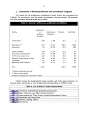Tabulation of Principal Results and Schematic Diagram The results for the employment multipliers for each project are summarized in Table A. For construction, only the indirect and induced jobs are counted. All figures in this table represent permanent new jobs created. Table A. Summary of Revenue and Employment Effects Expenditures or Revenues ($ million) Final Demand Multiplier Construction * 4.43 7.268 32.2 x Retail Stores ** Restaurants 18.5 2.6 19.927 25.075 368.6 65.2 252.5 48.7 Offices of lawyers Accounting, tax preparation Architectural, engineering Computer systems design services Consultants Advertising, public relations 0.93 0.79 1.32 1.51 1.07 1.36 15.514 19.986 14.372 16.963 16.582 16.531 14.4 15.8 19.0 25.6 17.7 22.5 5.3 9.2 6.7 9.2 6.7 5.3 581.1 343.6 Activity Total 32.51 Total Jobs Direct Jobs * Indirect and induced jobs only ** Sales are value added All figures calculated from unrounded numbers Table B shows the 6-digit NAICS codes used for each of the above activities. In several cases, there are 2 or more 6-digit codes corresponding to 1 RIMS II code. Table B. List of NAICS Codes Used in Model 236220 Commercial and Institutional Building Construction 443112 Radio, Television, and Other Electronics Stores 445110 Supermarkets and Other Grocery (except Convenience) Stores 446110 Pharmacies and Drug Stores 448120 Women's Clothing Stores 448210 Shoe Stores  5 448310 Jewelry Stores 451110 Sporting Goods Stores 452112 Discount Department Stores 453220 Gift, Novelty, and Souvenir Stores 722110 Full-Service Restaurants 541110 Offices of Lawyers 541211 Offices of Certified Public Accountants 541310 Architectural Services 541330 Engineering Services 541512 Computer Systems Design Services 541611 Administrative Management and General Management Consulting Services 541618 Other Management Consulting Services 541810 Advertising Agencies 541820 Public Relations Agencies If all the buildings in the proposed regional center were to be completely finished and occupied within two and a half years, the economic impact as measured by household earnings, demand for business services, utilities, maintenance and repair, and new supplier and vendor relationships is summarized in Table C. Table C. Summary Measures of Economic Impact for All Buildings in Regional Center Category All figures in thousands of dollars Household income from: Construction jobs Office space Retail space and restaurants Total Household Income Demand for professional and business support services Demand for utility services: electric, natural gas, and water Maintenance and repair construction New supplier/vendor relations created with manufacturers Total of these 4 categories Total $1,112 $4,871 $11,587 $17,570 $11,145 $711 $272 $1,291 $13,419  6 Household Earnings (Labor Income) The jobs created by the various components of the Coronado Canyons Building will subsequently create new sources of household income. The household income for the total jobs created by construction totals about $1.1 million. The household income for the total jobs created by the operation of the office space is about $4.8 million, and for the retail and restaurant space is about $11.6 million, for a total of about $17.6 million for this building. This income calculation comes from the RIMS II input-output model, which measures the average income per job by industry. The model calculations are based on the types of jobs that will be created within the regional center, with indirect/induced impacts allocated based on the types of commodity inputs required by the businesses that would potentially locate in the regional center. Demand for Business Services, Utilities, Maintenance and Construction, and New Supplier/Vendor Relationships Created with Manufacturers The total economic impact of the regional center from the supplier purchases and business relationships for the Coronado Canyons Building will create approximately $13.4 million in additional economic activity across the region. These supplier purchases are calculated from the indirect increase in output generated by the RIMS II model. It should be noted that some of these supplier industries might potentially locate within the regional center, and their economic output is included in this total. The estimate of supplier purchases is based on the commodity data in the RIMS II input-output model. This data specifies the amount and type of commodity input needed to maintain specific types of business operations. The model estimates the supplier purchases based on the types of jobs and number of jobs that will be created within the regional center. In addition, the model allocates the supplier purchases to businesses within the region, based on trade flow data from the U.S. Bureau of Economic Analysis. The regional center will create demand for business services including, professional services, management of companies, and administration and waste management services. The impact of this activity totals about $11.1 million annually. Most of this represents the direct output of the office space in the building. Utilities include services such as electricity, natural gas, and water and sewer facilities. The economic impact on utility services totals about $0.7 million. Maintenance and repair services include some building and construction activity on existing buildings. The regional center would create an economic impact of about $0.3 million within these sectors in the region. This figure is in addition to the $4.43 million in renovation construction that will be undertaken before the building is occupied.  7 New supplier/vendor relationships with manufacturers would create an economic impact of $1.3 million. Most of this represents the purchases of locally manufactured goods used in construction. 3. Introduction and Scope of Work Nevada California Regional Center, LLC plans to purchase a currently vacant mixed use commercial building located at 650 S. Green Valley Pkwy., Henderson, NV 89052, which is in Clark County. The building consists of four units, with first-floor retail space of about 74,760 square feet and second-floor office space of approximately 13,800 square feet. The building is located within the Green Valley Ranch master planned community, with close access to the Green Valley Corporate Center, Green Valley Ranch Resort and Casino, the District, and St. Rose Hospital. Section (4) contains a brief discussion of the RIMS II model. Section (5) presents the data for the principal economic parameters for this region for Clark County, compared to the statistics for the state of Nevada and the overall U. S. economy. Section (6) shows the location of Clark County area and explains why no other counties are included in the multiplier analysis. It also describes the location of the Coronado Canyons Building. Section (7) discusses the construction expenditures for renovation, and presents the economic impact of that activity. Results are shown for the increase in employment, output, and earnings, and the average level of output and earnings per new worker, for the 20 major industrial classifications calculated by the RIMS II model. Section (8) discusses the employment and revenue effects that will occur from the operations of the retail space and restaurants, and presents the economic impact tables for these operations. Section (9) provides similar material for the office space. The combined results for the entire project are summarized in Section (10).  8 4. Discussion of RIMS II Final Demand Methodology The following material has been condensed from the RIMS II User Handbook Introduction and General Comments Effective planning for public- and private-sector projects and programs at the State and local levels requires a systematic analysis of the economic impacts of these projects and programs on affected regions. In turn, systematic analysis of economic impacts must account for the inter-industry relationships within regions because these relationships largely determine how regional economies are likely to respond to project and program changes. Thus, regional input-output (I-O) multipliers, which account for inter-industry relationships within regions, are useful tools for conducting regional economic impact analysis. In the 1970s, the Bureau of Economic Analysis (BEA) developed a method for estimating regional I-O multipliers known as RIMS (Regional Industrial Multiplier System), which was based on the work of Garnick and Drake. In the 1980s, BEA completed an enhancement of RIMS, known as RIMS II (Regional Input-Output Modeling System), and published a handbook for RIMS II users. In 1992, BEA published a second edition of the handbook in which the multipliers were based on more recent data and improved methodology. In 1997, BEA published a third edition of the handbook that provides more detail on the use of the multipliers and the data sources and methods for estimating them. RIMS II is based on an accounting framework called an I-O table. For each industry, an I-O table shows the industrial distribution of inputs purchased and outputs sold. A typical I-O table in RIMS II is derived mainly from two data sources: BEA's national I-O table, which shows the input and output structure of nearly 500 U.S. industries, and BEA's regional economic accounts, which are used to adjust the national I-O table to show a region's industrial structure and trading patterns. Using RIMS II for impact analysis has several advantages. RIMS II multipliers can be estimated for any region composed of one or more counties and for any industry, or group of industries, in the national I-O table. The accessibility of the main data sources for RIMS II keeps the cost of estimating regional multipliers relatively low. Empirical tests show that estimates based on relatively expensive surveys and RIMS IIbased estimates are similar in magnitude. BEA's RIMS multipliers can be a cost-effective way for analysts to estimate the economic impacts of changes in a regional economy. However, it is important to keep in mind that, like all economic impact models, RIMS provides approximate order-ofmagnitude estimates of impacts. RIMS multipliers are best suited for estimating the impacts of small changes on a regional economy. For some applications, users may want to supplement RIMS estimates with information they gather from the region undergoing the potential change. To use the multipliers for impact analysis effectively, users must provide geographically and industrially detailed information on the initial  9 changes in output, earnings, or employment that are associated with the project or program under study. The multipliers can then be used to estimate the total impact of the project or program on regional output, earnings, and employment. RIMS II is widely used in both the public and private sector. In the public sector, for example, the Department of Defense uses RIMS II to estimate the regional impacts of military base closings. State transportation departments use RIMS II to estimate the regional impacts of airport construction and expansion. In the private-sector, analysts and consultants use RIMS II to estimate the regional impacts of a variety of projects, such as the development of shopping malls and sports stadiums. RIMS II Methodology RIMS II uses BEA's benchmark and annual I-O tables for the nation. Since a particular region may not contain all the industries found at the national level, some direct input requirements cannot be supplied by that region's industries. Input requirements that are not produced in a study region are identified using BEA's regional economic accounts. The RIMS II method for estimating regional I-O multipliers can be viewed as a three-step process. In the first step, the producer portion of the national I-O table is made region-specific by using six-digit NAICS location quotients (LQs). The LQs estimate the extent to which input requirements are supplied by firms within the region. RIMS II uses LQs based on two types of data: BEA's personal income data (by place of residence) are used to calculate LQs in the service industries; and BEA's wage-andsalary data (by place of work) are used to calculate LQs in the non-service industries. In the second step, the household row and the household column from the national I-O table are made region-specific. The household row coefficients, which are derived from the value-added row of the national I-O table, are adjusted to reflect regional earnings leakages resulting from individuals working in the region but residing outside the region. The household column coefficients, which are based on the personal consumption expenditure column of the national I-O table, are adjusted to account for regional consumption leakages stemming from personal taxes and savings. In the last step, the Leontief inversion approach is used to estimate multipliers. This inversion approach produces output, earnings, and employment multipliers, which can be used to trace the impacts of changes in final demand on and indirectly affected industries. Advantages of RIMS II There are numerous advantages to using RIMS II. First, the accessibility of the main data sources makes it possible to estimate regional multipliers without conducting relatively expensive surveys. Second, the level of industrial detail used in RIMS II helps avoid aggregation errors, which often occur when industries are combined. Third, RIMS II multipliers can be compared across areas because they are based on a consistent set  10 of estimating procedures nationwide. Fourth, RIMS II multipliers are updated to reflect the most recent local-area wage-and-salary and personal income data. Overview of Different Multipliers RIMS II provides users with five types of multipliers: final demand multipliers for output, for earnings, and for employment; and direct-effect multipliers for earnings and for employment. These multipliers measure the economic impact of a change in final demand, in earnings, or in employment on a region’s economy. The final demand multipliers for output are the basic multipliers from which all other RIMS II multipliers are derived. In this table, each column entry indicates the change in output in each row industry that results from a $1 change in final demand in the column industry. The impact on each row industry is calculated by multiplying the final demand change in the column industry by the multiplier for each row. The total impact on regional output is calculated by multiplying the final demand change in the column industry by the sum of all the multipliers for each row except the household row. RIMS II provides two types of multipliers for estimating the impacts of changes on earnings: final demand multipliers and direct effect multipliers. These multipliers are derived from the table of final demand output multipliers. The final demand multipliers for earnings can be used if data on final demand changes are available. In the final demand earnings multiplier table, each column entry indicates the change in earnings in each row industry that results from a $1 change in final demand in the column industry. The impact on each row industry is calculated by multiplying the final demand change in the column industry by the multipliers for each row. The total impact on regional earnings is calculated by multiplying the final demand change in the column industry by the sum of the multipliers for each row. Employment Multipliers RIMS II provides two types of multipliers for estimating the impacts of changes on employment: final demand multipliers and direct effect multipliers. These multipliers are derived from the table of final demand output multipliers. The final demand multipliers for employment can be used if the data on final demand changes are available. In the final demand employment multiplier table, each column entry indicates the change in employment in each row industry that results from a $1 million change in final demand in the column industry. The impact on each row industry is calculated by multiplying the final demand change in the column industry by the multiplier for each row. The total impact on regional employment is calculated by multiplying the final demand change in the column industry by the sum of the multipliers for each row.  11 The direct effect multipliers for employment can be used if the data on the initial changes in employment by industry are available. In the direct effect employment multiplier table, each entry indicates the total change in employment in the region that results from a change of one job in the row industry. The total impact on regional employment is calculated by multiplying the initial change in employment in the row industry by the multiplier for the row. Choosing a Multiplier The choice of multiplier for estimating the impact of a project on output, earnings, and employment depends on the availability of estimates of the initial changes in final demand, earnings, and employment. If the estimates of the initial changes in all three measures are available, the RIMS II user can select any of the RIMS II multipliers. In theory, all the impact estimates should be consistent. If the available estimates are limited to initial changes in final demand, the user can select a final demand multiplier for impact estimation. If the available estimates are limited to initial changes in earnings or employment, the user can select a direct effect multiplier.  12 5. Economic Parameters for Clark County This section is organized as follows. Table 5-1 shows the key economic parameters for Clark County and compares then with Nevada and the U.S. Table 5-2 show the labor force, employment, and unemployment statistics for Las Vegas, Clark County, and Nevada from 2000 through 2010. Table 5-1. Comparison of Clark County, Nevada, and the U.S. Category EMPLOYMENT STATUS Population 16 years and over In labor force Civilian labor force Employed Unemployed Armed Forces Not in labor force OCCUPATION Civilian employed population 16 + Management & professional Service occupations Sales and office occupations Farming, fishing, & forestry Construction, maintenance, repair Production & transportation INDUSTRY Civilian employed population 16 + Agriculture & mining Construction Manufacturing Wholesale trade Retail trade Transportation & utilities Information Finance, insurance & real estate Professional & administrative Educational services & health care Arts, entertainment, hotel, food svcs Other private services Clark County NV Nevada 1,423,938 998,060 989,412 917,302 72,110 8,648 425,878 100.0% 70.1% 69.5% 64.4% 5.1% 0.6% 29.9% 2,003,468 1,384,364 1,374,480 1,273,822 100,658 9,884 619,104 100.0% 69.1% 68.6% 63.6% 5.0% 0.5% 30.9% United States 238,764,455 157,465,113 156,225,077 146,266,253 9,958,824 1,240,036 81,299,342 % 917,302 243,258 250,434 235,890 630 105,465 81,625 100.0% 26.5% 27.3% 25.7% 0.1% 11.5% 8.9% 1,273,822 347,001 326,054 329,307 3,019 148,914 119,527 100.0% 27.2% 25.6% 25.9% 0.2% 11.7% 9.4% 146,266,253 51,064,301 25,084,498 37,252,708 997,997 13,612,976 18,253,773 100.0% 34.9% 17.1% 25.5% 0.7% 9.3% 12.5% 917,302 2,115 96,842 31,928 18,307 103,556 42,821 15,963 62,592 96,545 115,676 100.0% 0.2% 10.6% 3.5% 2.0% 11.3% 4.7% 1.7% 6.8% 10.5% 12.6% 1,273,822 20,152 132,098 57,897 28,004 151,241 62,421 21,560 81,270 128,205 170,598 100.0% 1.6% 10.4% 4.5% 2.2% 11.9% 4.9% 1.7% 6.4% 10.1% 13.4% 146,266,253 2,653,081 10,777,675 16,381,624 4,383,802 16,994,717 7,595,843 3,527,777 10,112,239 15,242,426 31,757,530 100.0% 1.8% 7.4% 11.2% 3.0% 11.6% 5.2% 2.4% 6.9% 10.4% 21.7% 257,223 39,040 28.0% 4.3% 309,995 51,654 24.3% 4.1% 12,904,517 7,092,352 8.8% 4.8% 100.0% 65.9% 65.4% 61.3% 4.2% 0.5% 34.1%  13 Public administration 34,694 3.8% 58,727 4.6% 6,842,670 4.7% INCOME AND BENEFITS Total households Less than $10,000 $10,000 to $14,999 $15,000 to $24,999 $25,000 to $34,999 $35,000 to $49,999 $50,000 to $74,999 $75,000 to $99,999 $100,000 to $149,999 $150,000 to $199,999 $200,000 or more Median household income (dollars) Mean household income (dollars) 684,605 35,790 25,892 58,746 68,720 107,273 144,646 99,108 90,548 29,599 24,283 56,696 72,696 100.0% 5.2% 3.8% 8.6% 10.0% 15.7% 21.1% 14.5% 13.2% 4.3% 3.5% 109.0% 101.7% 952,856 52,212 36,982 86,534 95,560 143,748 202,151 137,512 127,347 38,334 32,476 56,361 72,233 100.0% 5.5% 3.9% 9.1% 10.0% 15.1% 21.2% 14.4% 13.4% 4.0% 3.4% 108.3% 101.0% 113,101,329 8,149,557 6,141,047 12,049,123 11,718,207 16,028,909 21,251,695 14,015,215 13,921,120 4,954,443 4,872,013 52,029 71,498 100.0% 7.2% 5.4% 10.7% 10.4% 14.2% 18.8% 12.4% 12.3% 4.4% 4.3% Families Less than $10,000 $10,000 to $14,999 $15,000 to $24,999 $25,000 to $34,999 $35,000 to $49,999 $50,000 to $74,999 $75,000 to $99,999 $100,000 to $149,999 $150,000 to $199,999 $200,000 or more Median family income (dollars) Mean family income (dollars) Per capita income (dollars) 440,732 14,053 9,470 30,023 40,261 67,329 96,484 71,269 69,466 22,957 19,420 64,255 81,802 27,383 100.0% 3.2% 2.1% 6.8% 9.1% 15.3% 21.9% 16.2% 15.8% 5.2% 4.4% 101.4% 98.1% 99.3% 615,019 21,484 13,614 43,042 53,409 88,860 136,737 101,857 99,278 30,253 26,485 64,910 81,931 27,421 100.0% 3.5% 2.2% 7.0% 8.7% 14.4% 22.2% 16.6% 16.1% 4.9% 4.3% 102.4% 98.3% 99.4% 75,030,551 3,211,198 2,404,943 6,148,998 6,827,538 10,239,597 15,144,495 11,047,974 11,568,389 4,251,923 4,185,496 63,366 83,351 27,589 100.0% 4.3% 3.2% 8.2% 9.1% 13.6% 20.2% 14.7% 15.4% 5.7% 5.6% Median earnings for workers Median earnings for male full-time Median earnings for female fulltime 31,605 43,643 105.8% 95.8% 31,241 45,178 104.6% 99.2% 29,868 45,556 34,875 98.3% 34,724 97.9% 35,471 7.6% 10.8% 78.4% 81.8% 7.9% 11.3% 81.4% 85.6% 9.7% 13.2% PERCENTAGE BELOW POVERTY All families All people Note: in this table, the percentage figures in black are proportions of the total in that category, while the percentage figures in red are relative to the U.S. figures.  14 The occupational figures for Clark County show a larger than average proportion of employees in construction, with 10.6% of the workforce in that industry compared to 7.4% nationally, although that figure may diminish as the housing slump continues. The county has a very small manufacturing base -- 3.5% compared to 11.2% nationally. Of course the huge difference occurs in tourism – leisure time activities, hotels, and restaurants – with a whopping 28.0% of the workforce engaged in that sector, compared to 8.8% nationally. As a result, there are relatively fewer people employed in virtually all other sectors, with the biggest decrement in education and health care, with only 12.6% of the workforce employed there, compared to 21.7% nationally. In spite of the marketing slogan that “What happens in Vegas, stays in Vegas”, the city is not particularly wealthy; only 3.5% of the households have incomes of over $200,000 per year, compared to 4.3% nationally. However, there are also relatively few poor people, so median household income is 109% of the national average. Family income is only 101% of the national average, as many of the relatively affluent households are not families as defined by the Census. The poverty levels are well below average, and are about 2 percentage points below the U. S. figures. Table 5-2. Key Labor Market Statistics, Clark County, Las Vegas, and Nevada, 2000-2010 Labor Force Employed Unemployed Un Rate, % 2000 2001 2002 2003 2004 2005 2006 2007 2008 2009 2010 Clark County 727521 759562 783659 806062 830951 872410 911492 934560 960679 971430 969098 693933 717631 737301 762771 793908 833717 873249 891813 896809 847668 821597 33588 41931 46358 43291 37043 38693 38243 42747 63870 123762 147501 4.6 5.5 5.9 5.4 4.5 4.4 4.2 4.6 6.6 12.7 15.2 2000 2001 2002 2003 2004 2005 2006 Las Vegas 245183 256125 264315 271780 280014 269094 274709 233195 241159 247769 256328 266792 257161 262958 11988 14966 16546 15452 13222 11933 11751 4.9 5.8 6.3 5.7 4.7 4.4 4.3  15 2007 2008 2009 2010 276023 279201 282262 281753 263020 260070 245079 237541 13003 19131 37183 44212 4.7 6.9 13.2 15.7 2000 2001 2002 2003 2004 2005 2006 2007 2008 2009 2010 State of Nevada 1062845 1101020 1130780 1153910 1180314 1228339 1276387 1307321 1336309 1354126 1350309 1015221 1042182 1066477 1093507 1128223 1173425 1222277 1247491 1246696 1184431 1149537 47624 58838 64303 60403 52091 54914 54110 59830 89613 169695 200772 4.5 5.3 5.7 5.2 4.4 4.5 4.2 4.6 6.7 12.5 14.9 Nevada has been harder hit by the recession than any other state, with the result that the unemployment rate soared to 14.9% in 2010, meaning the entire state is a TEA. The unemployment rate in Clark County was even higher, at 15.2%, while for the city of Las Vegas the rate was 15.7%. There were more than 147,000 unemployed people in Clark County in 2010. 6. Maps of Area and Location of Building Figure 6-1 shows the map of Clark County, which is located at the southern tip of Nevada, wedged in between California and Arizona. It is basically a self-contained county; of the total reported workforce of 644,266 in 2000, 620,500 of those people were residents of the county. That 96.3% is an unusually high percentage. As a result, the multiplier estimates used throughout this report are based only on Clark County. Figure 6-2 shows the map of Henderson, NV, and Figure 6-3 shows the location of the Colorado Canyons building, which is at the southeast corner of S. Green Valley Pkwy and W. Horizon Ridge Pkwy  16 Figure 6-1. Map of Clark County Figure 6-2. Map of Henderson, NV  17 Figure 6-3. Location of Colorado Canyons Building 7. Economic Impact of Construction Expenditures for Renovation According to the developer, about $50 per square foot will be spent to renovate the building, so for a total of 88,560 square feet, that would be about $4.43 million. Even if the construction project takes less than two years, the indirect and induced jobs can be counted. On January 16, 2009, James W. McCament, Chief of USCIS, wrote a letter to Senator John Cornyn, which contained the following language: Indirect and induced jobs created as a result of construction jobs whether counted or not may be included in the job count. Even when the construction jobs may not be counted towards the job creation requirement, they do have indirect and induced impacts that are eligible to be included in the final job count because they are "continuous, permanent employment." The economic argument behind this logic may be summarized as follows. Consider a tax cut that is temporary (perhaps a rebate). It clearly provides some initial stimulus, but then it is not repeated. Nonetheless, the overall state of the  18 economy has improved; no one argues that real GDP drops back to its previous level once the rebate expires. Instead, the temporary stimulus has boosted overall demand; during the time of the rebate, money was spent, people were hired, and those benefits continued after the rebate period had passed. In this light, we can also look at a stimulus program (perhaps public works) which would be even more appropriate considering we are analyzing temporary investment. Public funds are expended for various projects over (say) one year, and when the projects are completed, the stimulus is not repeated. However, the economy is clearly better off because that stimulus has in fact created jobs, caused new workers to spend their paychecks, etc., which has a multiplier (or ripple) effect throughout the economy that does not disappear even after the public works funds have been expired. In fact, in the case of public works projects such as highways, railroads, utilities, etc. the argument is also made that the productive capacity of the economy has been increased, so the economy benefits from a supply-side as well as a demand-side stimulus. To the extent that overall capacity has increased, the economy is able to produce more as it gradually returns to a position of full employment. Tables 7-1 and 7-2 show the economic impact of the construction activity for renovating the building. Table 7-1. Increase in Employment, Output, and Earnings, $4.43 Million in Construction Expenditures, Indirect and Induced Jobs Only Industry Group Agriculture, forestry, fishing, Mining Utilities Construction Manufacturing Wholesale trade Retail trade Transportation and warehousing Information Finance and insurance Real estate and rental and leasing Professional and scientific services Management of companies Admin and waste mgmt services Educational services Health care and social assistance Arts, entertainment, and recreation Accommodation Food services and drinking places Other services Employment 0.0 0.1 0.2 0.3 2.3 1.1 7.1 1.3 0.6 1.3 2.7 3.4 0.3 2.5 0.5 3.0 0.6 0.5 2.4 1.7 Output 0 20 81 31 428 188 518 137 144 260 624 436 89 128 28 282 40 48 130 162 Earnings 0 5 15 12 97 59 181 51 31 66 50 190 37 53 11 135 13 14 41 50  19 Household Total 0.4 0 4 32.2 3774 1112 Table 7-1 shows there would be a total of 32 indirect and induced new jobs created by this activity, with an increase in output of about $3.8 million, and an increase in labor income of $1.1 million. Table 7-2 shows that the average output per new worker would be about $117,200, and average annual earnings would be about $34,500. Table 7-2. Output, and Earnings, $4.43 Million in Construction Expenditures, Indirect and Induced Jobs Only Industry Group Agriculture, forestry, fishing, Mining Utilities Construction Manufacturing Wholesale trade Retail trade Transportation and warehousing Information Finance and insurance Real estate and rental and leasing Professional and scientific services Management of companies Admin and waste mgmt services Educational services Health care and social assistance Arts, entertainment, and recreation Accommodation Food services and drinking places Other services Household Total Employment 0.0 0.1 0.2 0.3 2.3 1.1 7.1 1.3 0.6 1.3 2.7 3.4 0.3 2.5 0.5 3.0 0.6 0.5 2.4 1.7 0.4 Output/Empl 142.9 189.3 516.9 118.7 189.5 177.2 73.3 104.0 223.8 206.8 227.4 129.5 272.4 50.3 57.1 94.1 61.4 105.1 53.3 95.5 0.0 Earnings/Empl 0.0 49.4 96.0 45.4 42.7 56.0 25.5 38.4 47.5 52.2 18.1 56.4 112.5 20.8 21.8 45.1 20.5 31.1 16.9 29.2 9.7 32.2 117.2 34.5  20 8. Discussion of Revenue and Employment, and Economic Impact, for Retail Space and Restaurants The methodology used for determining the economic impact of retail jobs is as follows. First, the national figures for sales per square foot for 16 different categories of retail chain stores are taken from the 2009 Bizminer survey, as shown in Table 8-1. Second, these figures are adjusted for sales per square foot in Clark County. Third, these figures are multiplied by the projected number of square feet for each type of retail establishment, which provides revenue estimates. These are also shown in Table 8-1 for retail stores, and are estimated to be 70,000 square feet of stores plus 4,760 square feet for the restaurant, for a total of 74,760 square feet of retail space. Fourth, the retail sales (but not restaurant) figures are converted from sales to value added by multiplying by the average retail margin of 0.45; that step is necessary because in all input/output models, the trade sector figures for “output” are actually value added. Fifth, the value added figures for retail sales are multiplied by the RIMS II final demand multiplier of 19.93 for retail sales in Clark County, and the sales figures for restaurants are multiplied by 25.075. Those results are shown in Tables 8-3 and 8-4. Table 8-1. Calculation of Retail Sales for Coronado Canyons Building Category Auto parts, accessories Furniture, home furnishings Electronics and appliances Bldg materials Food and beverage Pharmacies Clothing stores Shoe stores Jewelry, luggage Sporting goods, hobby Books, magazines General merchandise Misc stores Total Key to Table 8-1. sal/emp Natl 151.9 191.6 224.1 239.6 190.2 247.6 123.9 127.1 191.4 135.5 119.3 208.9 131.1 sal/emp Clark 157.6 239.8 227 233.9 191.6 182 162.9 294.8 148.6 161.2 228.6 182.9 144.8 Ratio 1.038 1.07 1.194 0.976 0.874 1.389 1.282 1.541 1.136 1.35 1.094 1.07 1.104 Sales/sf Natl 198 243 769 281 559 911 329 354 783 234 238 548 175 Sales/sf Clark 206 260 918 274 489 1265 422 546 889 316 260 586 193 Square Feet Sales Mil $ 10 9.2 10 5 10 5 5 5 4.9 6.3 4.2 2.7 4.4 1.6 10 10 5.9 1.9 70 41.1  21 Sal/emp, Natl = sales per employee, national, $000s, 2007 Economic Census Sal/emp, Clark= sales per employee, Clark County, $000s, 2007 Economic Census Ratio = Col (2)/Col (1) Sales/sf, Natl = sales per square foot from 2009 Bizminer survey Sales/sf, Clark = sales per square foot for Clark County equals national * ratio Square Feet = assumed square feet for each type of sales in Spring Mountain building Sales = square feet times sales/sf for Clark County, Mil $ The sales per square foot for restaurants are based on data taken from the Retail Traffic Magazine website and shown in Table 8-2. According to these figures, restaurant sales for major chains average about $550 per square foot. Table 8-2. Sales of Restaurants by Major Chain Chain Cheesecake Factory P.F. Chang's Cracker Barrel Olive Garden Red Lobster Outback Steakhouse Macaroni Grill Carraba's Joe's Crab Shack Chili's California Pizza Kitchen Red Robin O'Charley's Longhorn Steakhouse Applebee's Ruby Tuesday Average Units 76 90 484 532 680 665 198 133 138 711 135 110 206 180 372 449 Average Annual Sq. Ft. Seats ($millions) 11,000 340 $11 6,700 215 $5.70 10,000 187 $4.10 8,000 235 $3.90 6,600 190 $3.70 6,200 247 $3.40 7,100 265 $3.30 6,650 255 $3.10 8,000 215 $3.10 5,400 210 $3 5,000 150 $2.90 6,400 200 $2.90 6,750 255 $2.80 5,100 190 $2.60 4,850 185 $2.20 5,100 205 $2.20 108,850 60 Sales $1,000 $851 $410 $488 $561 $548 $465 $466 $388 $556 $580 $453 $415 $510 $454 $431 $550 The retail sales revenue of $41.1 million, and the restaurant sales of $2.6 million, are entered in the RIMS II model, and the results are shown in the next two tables. Table 8-3. Increase in Employment, Output, and Earnings for $41.1 Million of  22 Retail Sales ($18.5 Million of Value Added) and $2.6 Million of Restaurant Sales Industry Group Agriculture, forestry, fishing, Mining Utilities Construction Manufacturing Wholesale trade Retail trade Transportation and warehousing Information Finance and insurance Real estate and rental and leasing Professional and scientific services Management of companies Admin and waste mgmt services Educational services Health care and social assistance Arts, entertainment, and recreation Accommodation Food services and drinking places Other services Household Total Employment 0.0 0.0 1.0 1.6 3.6 3.4 270.6 9.2 4.2 6.2 21.1 9.2 2.2 14.3 2.2 12.3 3.5 1.8 59.4 6.5 1.5 Output 2 2 508 187 663 604 19819 853 852 1286 3468 1022 592 744 130 1154 214 188 3173 635 0 Earnings 0 0 98 72 145 192 6912 357 207 327 310 482 244 300 50 553 70 57 1005 192 15 433.7 36096 11587 Table 8-3 shows that the operations from the retail stores and restaurants would create a total of 434 new jobs, with an increase in output of about $36.1 million, and an increase in household earnings of about $11.6 million. Table 8-4 shows that the average output (value added) per retail sales employee is about $73,200, and average annual earnings are about $25,500. For restaurants, the comparable figures are $53,400 for output and $16,900 for earnings; the latter figure excludes most tips. For all new workers, the comparable figures are $83,200 for output per worker and $26,700 for average annual earnings. Table 8-4. Output and Earnings per New Worker for $41.1 Million of Retail Sales  23 and $2.6 Million of Restaurant Sales Industry Group Agriculture, forestry, fishing, Mining Utilities Construction Manufacturing Wholesale trade Retail trade Transportation and warehousing Information Finance and insurance Real estate and rental and leasing Professional and scientific services Management of companies Admin and waste mgmt services Educational services Health care and social assistance Arts, entertainment, and recreation Accommodation Food services and drinking places Other services Household Total Employment 0.0 0.0 1.0 1.6 3.6 3.4 270.6 9.2 4.2 6.2 21.1 9.2 2.2 14.3 2.2 12.3 3.5 1.8 59.4 6.5 1.5 Output/Empl 112.7 176.3 499.6 119.1 186.1 177.0 73.2 93.2 202.7 208.0 164.2 111.5 272.2 52.2 58.6 94.0 60.5 104.9 53.4 97.7 0.0 Earnings/Empl 0.0 0.0 96.7 45.9 40.7 56.2 25.5 39.0 49.2 52.9 14.7 52.6 112.2 21.0 22.4 45.0 19.7 31.5 16.9 29.6 9.8 433.7 83.2 26.7 9. Discussion of Revenue and Employment, and Economic Impact, for Office Space We start this section by estimating the number of direct employees per square foot. The number of lawyers and similar professions per square foot for office buildings can be taken from data supply by the U.S. Energy Information Agency. As part of its comprehensive study on energy use, the Energy Information Agency prepares annual estimates on the amount of energy used by type and size of commercial building. This study also estimates the number of mean square feet per worker by type of building. Their figure for office buildings, 434 square feet per worker, is used in this study. The complete table from the EIA study is given below, in Table 9-1. Table 9-1. Estimates of Square Feet per Worker by Type of Building  24 All Buildings*................................ Building Floorspace (Square Feet) 1,001 to ................................ 5,001 to .............................. 10,001 to ............................ 25,001 to ............................ 50,001 to .......................... 100,001 to ........................ 200,001 to ........................ Over ................................. Number of Buildings (thousand) Total Floorspace (million square feet) Total Workers in All Buildings (thousand) Mean Square Feet per Building (thousand) Mean Square Feet per Worker Mean Hours per Week 4,645 64,783 72,807 13.9 890 61 2,552 6,789 9,936 2.7 683 57 889 6,585 7,512 7.4 877 61 738 11,535 10,787 15.6 1,069 67 241 8,668 8,881 35.9 976 72 129 9,057 8,432 70.4 1,074 80 65 9,064 11,632 138.8 779 89 25 7,176 6,883 289.0 1,043 100 7 5,908 8,744 896.1 676 115 386 9,874 12,489 25.6 791 50 226 1,255 1,430 5.6 877 107 297 1,654 3,129 5.6 528 86 129 3,163 6,317 24.6 501 59 8 1,905 3,716 241.4 513 168 121 1,258 2,600 10.4 484 52 142 5,096 2,457 35.8 2,074 167 443 4,317 3,463 9.7 1,246 59 824 12,208 28,154 14.8 434 55 277 3,939 2,395 14.2 1,645 50 71 1,090 1,347 15.5 809 103 370 3,754 1,706 10.1 2,200 32 622 4,050 3,667 6.5 1,105 55 597 10,078 4,369 16.9 2,306 66 79 1,738 1,819 21.9 956 63 5,000 10,000 25,000 50,000 100,000 200,000 500,000 500,000 Principal Building Activity Education ....................................... Food Sales ..................................... Food Service ................................. Health Care .................................... Inpatient ....................................... Outpatient .................................... Lodging .......................................... Retail (Other Than Mall).................. Office ............................................. Public Assembly ............................ Public Order and Safety ................ Religious Worship .......................... Service .......................................... Warehouse and Storage ............... Other .............................................. However, an additional adjustment should be made. The 434 square feet per person assumes that the professionals in those offices need space for customer  25 accommodations, which is indeed the case for lawyers and other professions such as advertising executives or public relations firms. However, for other types of businesses, the number of square feet per employee is substantially smaller, and the number of employees larger, since it is not necessary to have reception areas, conference rooms, and other similar amenities for customers. For example, data available on 10 web sites of companies who specialize in research and development reveals the following number of square feet per employee: 250, 215, 219, 230, 250, 200, 200, 300, 300 and 250 -- for an average of 245 square feet per employee. Hence a 100,000 square foot office building housing those types of businesses would have 408 employees, or 77% more than the example given above. In terms of office staffing and space requirements for computer programmers, the layout would probably be similar to a company such as Amazon or Google. Amazon states that it allocates 180 to 250 square feet per programming employee, although the higher number is reserved for senior level personnel. Google states that it allocates 150 to 200 square feet per programming employee. Other similar office arrangements, based on Internet data, also show figures of 150 to 200 square feet per employee. In terms of other professional offices, it is assumed that the average number of space per employee will be midway between the 250 square foot figure for civic organizations and the 434 square foot figure for lawyers and accountants, or 342 square feet per employee. That provides room for some conference and meeting rooms, but less space for luxurious lobbies and reception areas. That is the figure used in this study. Since the type of tenants that would occupy this office building is not yet known, we use a combination of six different types of professions, as shown below in Table 9-1. For the calculations in this table, it is assumed that the 434 sq ft/employee figures applies to lawyers and advertising/public relationship, the 342 sq ft/employee figure applies to architects/engineers and consultants, and the 250 sq ft/employee figure applies to accountants/tax preparers and computer system and design services. The total amount of office space is 13,800 square feet, and is assumed to be divided equally among the six professions, which is 2,300 square feet for each type of profession given below in Table 9-2. Table 9-2. Estimate of Job Creation for Office Space direct Category Offices of lawyers Accounting, tax preparation, bookkeeping, and payroll services Architectural, engineering, and related services Computer systems design services Consultants total Rev/e 175.3 FD mult 15.51 e/sqft 434 jobs 5.3 rev 0.93 Jobs 14.4 85.4 197 163.7 159.2 19.99 14.37 16.87 16.58 250 342 250 342 9.2 6.7 9.2 6.7 0.79 1.32 1.51 1.07 15.7 19.0 25.4 17.8  26 Advertising, public relations, and related services 257.3 16.54 434 Total Office 5.3 1.36 22.6 42.4 6.98 114.9 Key to Table 9-2. Rev/e, revenue per employees, Clark County, 2007 Economic Census, $000/yr FD mult = RIMS II Final Demand multiplier for Clark County e/sq ft = employees per 1000 sq ft, see previous table and associated commentary empl = employees, calculated as 2,300 sq ft divided by previous column rev = revenue, equals employees times revenue/employee, millions of $ jobs = RIMS II final demand multiplier times revenue All figures are calculated from unrounded numbers Table 9-3 and 9-4 show the economic impact of operations in 13,800 square feet of office space. Table 9-3. Increase in Employment, Output, and Earnings for 13,800 Square Feet of Professional Office Space Industry Group Agriculture, forestry, fishing, Mining Utilities Construction Manufacturing Wholesale trade Retail trade Transportation and warehousing Information Finance and insurance Real estate and rental and leasing Professional and scientific services Management of companies Admin and waste mgmt services Educational services Health care and social assistance Arts, entertainment, and recreation Accommodation Food services and drinking places Other services Household Total Employment 0.0 0.0 0.2 0.5 1.1 1.0 7.2 2.5 1.8 2.4 6.2 66.7 0.7 6.9 0.9 5.2 1.8 1.2 5.7 2.5 0.6 Output 1 1 122 55 199 172 528 242 355 501 1186 7620 186 329 49 485 116 128 305 245 Earnings 0 0 23 21 46 55 184 97 78 128 94 3425 77 142 19 232 37 38 96 73 6 115.0 12824 4871  27 Table 9-3 shows that the operations of the office space would create 115 new jobs. The increase in output would be about $12.8 million, and the increase in household earnings would be about $4.9 million. Table 9-4 shows that the average output per new worker would be about $115,000, and average annual earnings would be about $42,300. Table 9-4. Output and Earnings Per New Worker for 13,800 Square Feet of Professional Office Space Industry Group Agriculture, forestry, fishing, Mining Utilities Construction Manufacturing Wholesale trade Retail trade Transportation and warehousing Information Finance and insurance Real estate and rental and leasing Professional and scientific services Management of companies Admin and waste mgmt services Educational services Health care and social assistance Arts, entertainment, and recreation Accommodation Food services and drinking places Other services Household Total Employment 0.0 0.0 0.2 0.5 1.1 1.0 7.2 2.5 1.8 2.4 6.2 66.7 0.7 6.9 0.9 5.2 1.8 1.2 5.7 2.5 0.6 Output/Empl 157.5 150.7 511.1 118.7 183.1 177.0 73.2 95.9 203.0 207.1 192.5 114.3 272.0 47.3 57.4 94.0 63.3 105.4 53.4 98.1 0.0 Earnings/Empl 0.0 24.0 95.9 45.2 42.0 56.2 25.5 38.4 44.7 52.8 15.2 51.4 112.4 20.4 22.4 45.0 20.3 31.4 16.9 29.3 10.2 115.0 111.5 42.3  28 10. Summary Statistics for Entire Project The figures shown in Tables 10-1 and 10-2 are the summary of the tables presented in Sections (7), (8), and (9) and hence are shown for ease of exposition. Table 10-1. Increase in Employment, Output, and Earnings, Renovation and Operation of Colorado Canyons Building Industry Group Agriculture, forestry, fishing, Mining Utilities Construction Manufacturing Wholesale trade Retail trade Transportation and warehousing Information Finance and insurance Real estate and rental and leasing Professional and scientific services Management of companies Admin and waste mgmt services Educational services Health care and social assistance Arts, entertainment, and recreation Accommodation Food services and drinking places Other services Household Total Employment 0.0 0.1 1.4 2.3 6.9 5.4 284.9 13.0 6.6 9.9 30.0 79.2 3.2 23.8 3.6 20.4 6.0 3.5 67.5 10.7 2.5 Output 3 24 711 272 1291 964 20865 1231 1351 2047 5278 9078 867 1200 207 1921 370 365 3608 1043 0 Earnings 0 5 136 105 287 306 7277 504 316 520 453 4097 358 495 80 920 120 109 1143 315 25 581.0 52695 17570 Table 10-1 shows there will be a total of 581 new jobs created from the renovation and operations of the Coronado Canyons building. The increase in output will be about $52.7 million, and the increase in household earnings will be about $17.6 million. Table 10-2 shows that the average output per new workers will be about $90,700, and average annual earnings will be about $30,200.  29 Table 10-2. Output and Earnings Per New Worker, Renovation and Operation of Colorado Canyons Building Industry Group Agriculture, forestry, fishing, Mining Utilities Construction Manufacturing Wholesale trade Retail trade Transportation and warehousing Information Finance and insurance Real estate and rental and leasing Professional and scientific services Management of companies Admin and waste mgmt services Educational services Health care and social assistance Arts, entertainment, and recreation Accommodation Food services and drinking places Other services Household Total Employment 0.0 0.1 1.4 2.3 6.9 5.4 284.9 13.0 6.6 9.9 30.0 79.2 3.2 23.8 3.6 20.4 6.0 3.5 67.5 10.7 2.5 Output/Empl 123.8 186.2 503.5 118.9 186.7 177.0 73.2 94.8 204.8 207.6 175.8 114.6 272.1 50.5 58.1 94.0 61.5 105.1 53.4 97.5 0.0 Earnings/Empl 0.0 43.0 96.5 45.7 41.6 56.1 25.5 38.8 47.8 52.8 15.1 51.7 112.3 20.8 22.3 45.0 20.0 31.4 16.9 29.5 9.9 581.0 90.7 30.2