تحليل و توسعه مسئله رؤيت پذيري غيرخطي براي سيستم هاي محرکه الکتريکي

Modeling, Verification and Control of Asynchronous Motor (Induction Motor) Vahab Rostampour Ali Javadizadeh Umair javad Nihat Ozlü Department of Automation and Control Engineering, Politecnico di Milano, Italy Laboratory supervisor: Dr. Alan Facchinetti Dr. Alberto Bezzolato  Outline  Introduction  Definition of Matlab/Simulink  Induction Motor Model  Estimators  Controllers  Verification  Controller *  Observers *  Conclusion 2 * Fulfill in theory base  Introduction 3 • Due to enhanced and improved design of microprocessors and DSPs and their computational efficiency in the field of Electrical drive control also their compatibility with each other enable to achieve great success in the efficient control of AC drive with improved results in power dissipation. • Thanks to the very well known vector controls schemes which led to these achievements (Field Oriented Control-FOC). • In spite of linear dynamical systems, observability analysis is a very difficult task for nonlinear dynamical systems. • Observable systems, linear or nonlinear, do not show same behaviors with different observers. • Estimating the state of some systems are easier than other systems with a same type of observer.  Model of Induction motor 4 • The objective of Field Orientated Control (FOC) is to control the stator currents represented by a vector. The control is based on the creation of a time invariant system which works on two coordinates namely (d and q coordinates). Transformation is required to convert a three phase time dependent system into a system of d-q axis. • This transformation results a control in which the two components (d-q) of stator current acts separately on the rotor flux and torque and thus the FOC control allows us to control the induction motor.  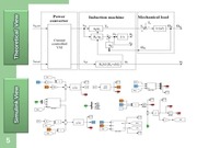5 Simulink View Theoretical View  Model of Estimatores • Current-Voltage Estimator Theoretical View The inputs used to design this estimator are stator voltages and currents only. Flux of stator is calculated from integration operation on voltages as shown below, and the rotor flux is calculated from stator currents and stator flux calculated. 6 Simulink View  Model of Estimatores • Current-Speed Estimator Theoretical View The inputs for this type of estimator are phase current and mechanical speed. The design of inverter is shown below 7 Simulink View  Model of Estimatores • Double Estimator Simulink View The two observers can be joined through a closed-loop leading to a new observer that minimizes the errors of the two original observers. 8  Model of Controllers • Current Loop Controller Theoretical View The closed loop transfer function: 9 Simulink View  Model of Controllers • Speed Loop Controller Theoretical View The closed loop transfer function: 10 Simulink View  Verification • Model results: Torque 11 Speed  Verification • Estimators results: 12  Verification • Controllers results: Vq,d 13 Vq,d (es)  Classical Controller (PID) • Current Controller (inner loop): num = [0 1]; den = [Lks Rks]; G1 = tf(num,den); %plant, open loop system Fc=100; %[Hz] Wc=2*pi*Fc; Kp_i=Wc*Rks; Ki_i=(Rks*Kp_i)/Lks; T_i=Kp_i/Ki_i; num=[Kp_i*(T_i) Kp_i]; den=[1 0]; C=tf(num,den); % Controller CL = feedback(G1*C,1); %closed loop system 14  15  Classical Controller (PID) • Speed Controller (outer loop): num = [0 1]; den = [J 0]; G2 = tf(num,den); %plant Fw=10; %[Hz] Ww=2*pi*Fw; Kp_w=Ww; Ki_w=(Kp_w)/J; T_w=Kp_w/Ki_w; num=[Kp_w*(T_i) Kp_w]; den=[1 0]; C2=tf(num,den); % Controller CL2 = feedback(G2*C2,1); %closed loop system 16  17  Advance Controller (MPC) Model Base Predictive Control 18  Continuous time LTI systems  x(t )  Ax(t )  Bu (t )   y (t )  Cx(t )  Du (t ) System’s model: Luenberger observer: xˆ  Axˆ  L( y  Du  Cxˆ )  Bu Theorem 1. In the design of Luenberger observer if the observer poles are considered in different places: a) Estimation error energy caused by measurement errors has an upper bound which depends on the norm of the observer gain: xˆ 19 2  y  (P ) 2 Min Re al (aˆi ) i L 2  Continuous time LTI systems b) Estimation error energy caused by model uncertainties in matrix A has an upper bound presented below: e (t ) 2  A  P  2   P1  B 2 Min Re al (aˆi ) Min Re al (ai ) i i A  P11D1P1 , D1  diag (ai ) Aˆ  A  LC  P 1DP , D  diag (aˆi )   P1  : condition number of P1   P  : condition number of P 20 u (t ) 2  Discrete time LTI systems  xk 1  Axk  Buk   yk  Cxk  Duk System’s model: Luenberger observer: xˆk 1  ( A  LC ) xˆk  L( yk  Duk )  Buk Theorem 2. In the design of Luenberger observer if the observer poles are considered in distinct places: a) Estimation error energy caused by measurement errors has an upper bound which depends on the norm of the observer gain: xˆ k 21 2  L 2 Min 1  aˆi i  y k 2  Discrete time LTI systems b) Estimation error energy caused by model uncertainties in matrix A has an upper bound presented below: e k 2  A  P  2 Min 1  aˆi i   P1  B 2   Min 1  a     P  A i i 1 A  P11D1P1 , D1  diag (ai ) Aˆ  A  LC  P 1DP , D  diag (aˆi )   P1  : condition number of P1   P  : condition number of P 22 2  uk 2  Kalman filter: an optimal estimator  Dependence of the observer gain on the observer poles  Dependence of the upper bound on the observer poles  An optimization criteria is required to specify the observer poles Kalman filter is an optimal estimator: Process model: Measurement model: Assumptions: Initial conditions: Covariance updating: Kalman gain: Estimation updating: 23 x(t )  Ax(t )  G (t ) z (t )  Hx(t )  v(t ) x(0) ( x0 , P0 ),  (0, Q), v P(0)  P0 , xˆ (0)  x0 (0, R) P(t )  AP  PAT  PH T R1HP  GQGT K (t )  P(t ) H T R 1 xˆ (t )  Axˆ (t )  K (t )  z(t )  Hxˆ(t )  Kalman filter for discrete systems Process model: Measurement model: Assumptions: Initial conditions: Time updating: xk 1  Ak xk  Bk uk  Gk k zk  H k xk  vk x0 ( x0 , Px0 ), k (0, Qk ), vk (0, Rk ) P0  Px0 , xˆ0  x0 xˆk1  Ak xˆk  Bk uk Pk1  Ak Pk AkT  Gk Qk GkT Measurement updating: 24   Pk 1   P   k 1 1  H R H k 1   T 1 k 1 k 1  1 xˆk 1  xˆk1  Pk 1H kT1Rk11 zk 1  H k 1 xˆk1   Comparative observability index Definition 1. Consider continuous time LTI systems with model uncertainties and measurement errors which are modeled in the form: x(t )  ( A  A) x(t )  Bu (t )  G (t ) y(t )  Cx(t )  y(t )  v(t ) Suppose that the steady state Kalman filter is designed to estimate the state of these systems. Comparative observability Index of these systems are defined as:    P1   (P )   L   B A 1 2 2 2 2 Min Re al (aˆi )  Min Re(ai )    P1  A 2 i i  A system is more observable than other systems if it has less observability Index.  25        Comparative observability index Definition 2. Consider discrete time LTI systems with model uncertainties and measurement errors which are modeled in the form: xk 1  ( A  A) xk  Buk  Gk yk  Cxk  yk  vk Suppose that the steady state Kalman filter is designed to estimate the state of these systems. Comparative observability Index of these systems are defined as:   (P )  L   B 1 2 2 Min  1  (aˆi )   i  26  (P1 ) 2  Min 1  a     P  A  i i 1 2  A 2    A system is more observable than other systems if it has less observability Index.  Generalization to nonlinear systems based on EKF Process model: Measurement model: Assumptions: Initial conditions: x  f  x, u, t   G (t ) z  h  x, t   v x(0)  x0 , P0  ,  (t )  0, Q  , v(t )  0, R  P(0)  P0 , xˆ (0)  x0 Covariance updating: P  A  xˆ, t  P  PAT  xˆ, t   GQGT  PH T  xˆ, t  R 1H  xˆ, t  P A  x, t   Kalman gain: Estimation updating: 27 f  x, u, t  x K  PH T  xˆ, t  R 1 , H  x, t   h  x, t  x Implementation?? xˆ  f  xˆ, u, t   K  z  h  xˆ, t   Generalization to nonlinear systems based on EKF The structure of the EKF is: 28  P  A  xˆ, t  P  PAT  xˆ, t   GQG T  PH T  xˆ, t  R 1H  xˆ, t  P  T 1 ˆ ˆ ˆ  z  z  h  xˆ, t   x  f x , u , t  PH x , t R      P(0)  P0 , xˆ (0)  x0 y  xˆ  Steady state filter is meaningless.  We are not easily able to find an upper bound for the estimation error due to measurement error.  Comparing the observability of nonlinear systems with EKF based on less sensitivity to measurement error is definable but is not easily computable. Changing the structure of the observer  H-infinity filtering Different views on H-infinity filtering: 1) H-infinity optimal controller 2) Minimizing the energy of exogenous signals in the estimation of variables The first view: J : sup L2 0,  29 z  zˆ  2 2 2 2 2  H-infinity filter: a robust estimator Second view: Cost function: Suboptimal condition: Estimation updating: Filter gain: J E    T e  edt  E  x(0)  xˆ (0) 2 P01   x  xˆ   x  xˆ  dt T x  xˆ S dt  2   2 Q 1 dt   v 2 R 1 2 dt xˆ  Axˆ  Bu u  K (t )  y  Cxˆ  K (t )  P(t )C T D T R 1D 1 Covariance updating: P(t )  AP(t )  P(t ) AT  B QBT  K (t )CP(t ) 30 P(t )  AP(t )  P(t ) AT  B QBT  K (t )CP(t )   2 P(t ) SP(t )  Conclusion 31  32 Torque Speed  Thanks for your attention 33