Biomedical Semantic Similarity

Evolutionary algorithm based on different semantic similarity functions for synonym recognition in the biomedical domain José M. Chaves-González, Jorge Martínez-Gil University of Extremadura. Escuela Politécnica, 10003, Cáceres, Spain. {jm, jorgemar}@unex.es Abstract Computing accurately the semantic similarity between terms represents an important challenge in the semantic web field. The problem here is the lack of appropriate dictionaries for specific and dynamic domains, such as the biomedical, financial or any other particular field. In this article we propose a new approach which uses different existing semantic similarity methods to obtain precise results which are very close to human judgments in the biomedical domain. Specifically, we have developed an evolutionary algorithm which uses information provided by different semantic similarity metrics. The results provided by our system have been validated using several medical datasets and different sets of similarity functions. We adopt the Pearson correlation coefficient as measure of the strength of the relation between human ratings of similarity and computation values. The proposed approach obtains the best results of correlation with regard to human judgments in comparison with other relevant similarity functions used in the mentioned domains. Index terms Semantic similarity, evolutionary computation, semantic web, synonym recognition, differential evolution I. Introduction With the increase of large collections of data resources on the World Wide Web (WWW), the study of web semantic techniques [1] has become one of the most active areas for researchers. The notion of semantic web expresses the aspiration to organize the available resources on basis of semantic information in order to facilitate its efficient processing. Related to this, the study of semantic similarity [2] between text expressions is a very relevant problem for certain applications in some specific fields, such as data integration  [3], query expansion [4] or document classification [5] (among others), because they need semantic similarity computation for working appropriately. On the other hand, semantic similarity measurements are usually performed using some kind of metrics [6]. The most common of those metrics are semantic similarity measures which are a kind of text based metrics resulting in a similarity or dissimilarity score between two given text strings to be compared. A semantic similarity measure provides a floating point number between 0 (total dissimilarity) and 1 (complete similarity). Most of the existing works have reached a high level of accuracy when solving datasets containing general purpose terms [7]. The majority of these works describe approaches which use large and updated dictionaries [6]. However, most of them often fail when dealing with expressions not covered by these dictionaries. In this work, we propose a new technique which beats a wide range of semantic similarity measurement methods. This technique consists of using an evolutionary algorithm which smartly combines the information provided by several classical semantic similarity functions. Thus, the evolutionary algorithm works as a high level heuristics which was designed with the purpose of improving the results obtained by using each individual similarity function. Therefore, in order to validate our proposal, we use some datasets belonging to the biological domain, where classical algorithms do not usually get the optimal results. The rest of this work is organized as follows: Section II elaborates on the work carried out on the problem and approaches handled in this paper. Section III describes the problem and the proposed solution. The methodology followed in all the experiments and the results obtained are presented and discussed in Section IV. Finally, conclusions and future lines of research are explained in the last section. II. Previous Work Semantic similarity measurement has traditionally been an active research area in the Natural Language Processing (NLP) field [8]. The reason is that the capability for synonym recognition is a key aspect in human conversations. However, with the quick development of the semantic web, researchers from this field have turned their attention to the possibility to adapt these techniques for making easier the discovery of resources from the WWW [9]. In this way, a user who is looking for cars can obtain results including terms such as automobiles, vehicles, and so on. For this reason, a number of publications which work in the intersection of NLP and semantic web have been developed over the last years [10].  On the other hand, a first approach for measuring semantic similarity between words could consist of computing the Euclidean distance (which is one of the most popular metrics in a lot of cultures) between the words. However, Euclidean distance is not appropriate for all types of data or patterns to be compared. For example, this kind of metrics is not appropriate to compute the distance between word meanings. For this reason, most of the previous works have been focused on designing new semantic similarity measures. Traditionally, these new semantic similarity measures use some kind of dictionaries in order to compute the degree of similarity between the words being compared. Some examples of these dictionaries are WordNet [6], MeSH (Medical Subject Headings) [7] and UMLS (Unified Medical Language System) [12]. These measures can be classified into three main categories: Path-based Measures which take into account the position of the terms in a given dictionary. If a word has two or more meanings, then multiple paths may exist between the two words. A problem for this approach is that it relies on the notion that all links in the taxonomy represent uniform distances. Information Content Measures. According to Pedersen et al. [6] information content measures are based on frequency counts of concepts as found in a corpus of text. Within this kind of measures, higher values are associated with more specific concepts (e.g., pitch fork), while those with lower values are more general (e.g., idea). Feature based Measures which measure the similarity between terms as a function of their properties or based on their relationships to other similar terms in a dictionary. In general, it is possible to estimate semantic similarity according to the amount of common features. An example of feature could be the concept descriptions retrieved from dictionaries. The problem of traditional semantic similarity metrics is that there are several fields where it is not easy to find complete and updated dictionaries. We focus on the biomedical domain. Related to the problem of semantic similarity measurement in this domain, several works have been proposed in recent years. For instance, Pirró [7] proposed a new information content measure using the MeSH biomedical ontology. Our study improves the results obtained in this study using a combination of several similarity functions. Experimental evaluations indicated that the proposed metrics improved the existing results for a given benchmark dataset. Nguyen and Al-Mubai [11] also proposed an ontology-based semantic similarity measure and applied it into the biomedical domain. The proposed measure is based on the path length between the concept nodes as well as the depth of the terms in the ontology hierarchy tree. Our results in this case are also closer to human judgment. Finally, Pedersen et al. [12] implemented and evaluated a variety of semantic similarity measures based on ontologies and terminologies found in the Unified Medical Language System (UMLS) obtaining very good results. Our results  are better also in this case because we combine the results from other proposals, and we obtain again more precise results as will be explained in the following sections. III. Differential Evolution for Synonym Recognition In this section we describe, on the one hand, the problem we have tackled in this paper and, on the other hand, the details of the solution proposed to solve it. Related to this, we explain both our evolutionary approach and the different methods which give support to the system developed. 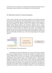Our approach is based on the similarity result provided by different atomic similarity functions. The evolutionary algorithm works as a hyperheuristics which assigns different coefficient values to the results of similarity calculated by the pool of functions which are included in the system. Thus, although all the functions (or metrics) are taken into account to provide the final semantic similarity of a specific term pair, the more similar to the human expert will possibly have at the end of the process the highest coefficients. Fig. 1 shows the working diagram of the proposed approach. Fig. 1. Working diagram of the proposed approach The differential evolution (DE) algorithm [13] was chosen among other candidates because after a preliminary study, it was proved that it obtained very competitive results for the problem tackled. The reason is in the way in which the algorithm makes the solution evolve. Due to our system can be considered a hyper-heuristics (HH) which uses the differential evolution (DE) to assign to each similarity function a coefficient which modifies its importance in the whole system, we have called our proposal HH(DE). 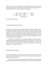Differential evolution performs the search of local optima by making small additions and subtractions between the members of its population (see Section III.C), and this feature fits perfectly to the problem, because the algorithm works with the scores provided by the similarity functions (Fig. 1). In fact, the individual is defined as an array of floating point  values, s, where s(fx) is the coefficient value which modifies the result provided by the similarity function f. Fig. 2 illustrates the solution encoded. This floating point value is between MIN and MAX, which is a parameter of the algorithm. Fig. 2. Individual representation A. The Synonym Recognition Problem Given two text expressions a and b, the problem addressed consists of trying to measure the degree of synonymy between them. The problem of synonym recognition usually extends beyond synonymy and involves semantic similarity measurement. According to Bollegala et al. [14], a certain degree of semantic similarity can be observed not only between synonyms (e.g. lift and elevator), but also between metonyms (e.g. car and wheel), hyponyms (leopard and cat), related words (e.g. blood and hospital) as well as between antonyms (e.g. day and night). Therefore, we are looking for a computational algorithm which may provide a floating point number indicating automatically the notion of similarity. A value of 0 will stand for not similarity between the (set of) words to be compared, while a value of 1 will indicate that the (set of) words share exactly the same meaning. A more detailed explanation can be found in Section IV. B. Semantic Similarity Metrics If we look at the literature, we can find a lot of similarity metrics. In this section we are going to present the similarity metrics that we use as the input for the hyper-heuristic algorithm developed (see Fig. 1). In Table I the most relevant similarity metrics are summarized according to their classification. The first column indicates the general type of the function. Second column  contains the similarity metrics and a reference in which it is possible to obtain more detailed information. Finally, the third column includes a brief explanation of the metrics. Table I. Classification of the most relevant similarity metrics. Type Similarity function and reference Path Length (PATH) [6] Leacock & Chodorow (LCH) [15] Path based measures Wu & Palmer (WUP) [16] Hirst & St-Onge (HSO) [17] Resnik (RES) [18] Information content measures Jiang & Conrath (JCN) [19] Lin (LIN) [20] Adapted Lesk (LESK) [21] Feature based measures Gloss Vector (vector) [22] Gloss Vector (pairwise modified) (vector_pairs) [6] Brief description It is inversely proportional to the number of nodes along the shortest path between the words. It can be computed as -log (length / (2 * D)), where length is the length of the shortest path between the two words and D is the maximum depth of the taxonomy. It considers the depths of the two terms in the taxonomies, along with the depth of the LCS (least common subsumer). The formula is: score = 2*depth(LCS) / (depth(s1) + depth(s2)). It finds lexical chains linking the two word senses. It computes the information content of the LCS. It can be computed in the following way: 1 / IC(term1) + IC(term2) - 2 * IC(LCS), where IC refers to information content. It can be computed as follows: 2 * IC(LCS) / (IC(term1) + IC(term2)). The similarity score is the sum of the squares of the overlap lengths. It works by forming second-order co-occurrence vectors from the glosses or WordNet definitions of concepts. This metrics forms separate vectors corresponding to each of the adjacent glosses. The main advantage of the path based measures is that they are very simple to interpret and implement. On the contrary, this kind of measures needs rich taxonomies,  only works with nodes belonging to these taxonomies, and only the relation is-a can be taken into account. The advantage of the Information Content measures is that use empirical information from real corpora. The problem is that only works with nodes (nouns) belonging to these taxonomies, and only is-a relationships can be considered. On the other hand, Feature based measures do not require underlying structures and use implicit knowledge from real large corpora. As a disadvantage, the definitions of the terms can be short, and moreover, the computation can be very intensive in the most of the cases. C. The Differential Evolution algorithm Differential Evolution (DE) heuristics [13] is a population based Evolutionary Algorithm (EA) used for function optimization. Due to its simplicity and effectiveness, DE has been applied to a large number of optimization problems in a wide range of domains [23]. Its key idea is based on the generation of new individuals by calculating vector differences between other randomly-selected solutions of the population. The algorithm has been carefully configured and adapted to the problem managed in our study, as will be explained in Section IV. For this reason, among the different variants of the algorithm [24], it was chosen the DE/best/1/bin version, because it provided more competitive results than other versions. The notation (DE/best/1/bin) indicates the way in which the crossover and mutation operators work. Thus, the DE developed includes binomial crossover (bin) and it only uses one (/1/) difference vector in the mutation process of the best solution of the population (best). Algorithm 1 shows an outline of the algorithm developed. Algorithm 1. Pseudo-code for the DE algorithm 1: generateRandomPopulation (population) 2: calculateFitness (population) 3: while (stop condition not reached) do 4: for (each individual of the population) 5: selectIndividuals (xTarget, xBest, xInd1, xInd2) 6: xTrial ← diffMutation (xBest, F, xInd1, xInd2) 7: xTrial ← binCrossOver (xTarget, xTrial, CrossProb) 8: calculateFitness (xTrial) 9: updateIndividual (xTarget, xTrial) 10: endfor 11: endwhile 12: return bestIndividual (population)  The algorithm starts with the random generation of the population (line 1) through the assignment of a random coefficient to each gene of the individual (see Fig. 2). Then, the fitness of each individual will be assigned using the Pearson correlation [25] with the values given by the human expert for all the word pairs of the specific dataset used in the experiment. This value of correlation, corr(X,Y), indicates the quality of the generated solutions and it is defined as expressed in equation 1 (see [25] for a detailed explanation of this equation). The result of this measure is a floating point value between +1 (perfect positive linear correlation) and -1 (perfect negative linear correlation). The result indicates the degree of linear dependence between the variables X (the human expert opinion) and Y (the solution evaluated). The closer to either -1 or +1, the stronger the correlation between variables and the higher the quality of the solution generated. On the other hand, if the result gets closer to 0, it means that the variables are closer to be uncorrelated, and therefore the solution is considered of poor quality. corr( X , Y )  cov( X , Y )  XY  E[( X   X )(Y  Y )]  X Y (1) After the evaluation of the whole population (line 2), each individual will be processed (line 4) to try to improve it. The first thing to do is to select four solutions (line 5). xTarget and xBest are the solution which is being processed and the best solution found, at that precise moment, respectively. xInd1 and xInd2 are two solutions different from xTarget and xBest chosen randomly. After that, the mutation operation is performed according to the following expression: xTrial ← xBest + F · (xInd1 – xInd2). This operator generates the xTrial individual which will be compared to the xTarget after the mutation and crossover operations (line 9). The parameter F [0, 2] establishes the mutation which is going to suffer the best solution, xBest. After the mutation, the xTarget and xTrial individuals are crossed using a binary crossover [26] according a certain crossover probability, crossProb  [0, 1]. The obtained individual is evaluated (equation 1) to check its quality (line 8) and finally will be compared with the xTarget solution. The best individual, or the best set of coefficients which modifies the metrics used by the system (Fig. 1), will be saved in the xTarget position and the other will be discarded. This process is repeated for each individual in the population (line 4) while the stop condition is not satisfied (line 3). In our case, the stop condition is a certain number of generations which is also an algorithm parameter to be configured (see Section IV.A). At the end of the process, the best individual, or set of coefficients (Fig. 2) which provides the best similarity results for the dataset which is being tackled, is returned as final result of our system (line 12).  IV. Experiments and Results In this section we summarize the main experiments and the results obtained in our study. We have used different similarity metrics and biomedical datasets to test the proposed system. A. Methodology All the experiments performed have been carried out under the same conditions: an Intel Xeon 2.33 GHz processor and 8 GB RAM. On the software side, we have used the GCC 4.1.2 compiler on a Scientific Linux 5.3 64 bits OS. Since we are dealing with a stochastic algorithm, we have carried out 100 independent runs for each experiment performed. Results provided in the following subsections are average results of these 100 executions. It is important to point here that the use of the arithmetic mean is a valid statistical measurement because the results obtained follow a normal distribution (a pvalue greater than 0.05 for the Shapiro-Wilk test confirms this fact [27]). Moreover, all the results present an extremely low dispersion, since the standard deviation for all the experiments is lower than 10-15, so results can be considered statistically reliable. In the following subsection we will discuss the results obtained with the different experiments using different similarity metrics and different word datasets, but before doing this, it is necessary to present the parameter setting for the algorithm developed. This configuration is very relevant, since the quality of the results obtained by the final system depends largely on the accuracy of this adjustment. Therefore, we performed a complete and precise parameter study for each parameter. All the results presented in the following subsections have been obtained using the same parameter setting, which is summarized in Table II. Table II. Optimal parameter setting. Parameter Population size Mutation factor, F Crossover probability, crossProb Max generations MIN, MAX Optimal value 100 0.5 0.1 100 -100, 100