Top-k Matching Queries for Filter-Based Profile Matching in Knowledge Bases

Top-k matching queries for filter-based profile matching in knowledge bases⋆ Alejandra Lorena Paoletti, Jorge Martinez-Gil, and Klaus-Dieter Schewe Software Competence Center Hagenberg, Hagenberg, Austria {Lorena.Paoletti, Jorge.Martinez-Gil, kd.schewe}@scch.at Abstract. Finding the best matching job offers for a candidate profile or, the best candidates profiles for a particular job offer, respectively constitutes the most common and most relevant type of queries in the Human Resources sector. This technically requires to investigate top-k queries on top of knowledge bases and relational databases. We propose in this paper a top-k query algorithm on relational databases able to produce effective and efficient results. The approach is to consider the partial order of matching relations between jobs and candidates profiles together with an efficient design of the data involved. In particular, the focus on a single relation, the matching relation, is crucial to achieve the expectations. 1 Introduction The accurate matching of job applicants to position descriptions and vice versa is of central importance in the Human Resources (HR) domain. The development of data or knowledge bases (KB) and databases to which job descriptions and curricula vitae (CV) can be uploaded and which can be queried effectively and efficiently by both, employers and job seekers is of high importance. Finding the best matching job offers for a candidate profile or, the best candidate profiles to a particular job offer respectively, constitute the most common and most relevant type of query, which technically requires to investigate top-k queries on top of knowledge bases and relational databases. A profile describes a set of skills either, a person posses detailed in form of a CV or, described in a job advertisement through the job description. Profile matching concerns to measure how well a given profile matches a requested profile. Although, profile matching is not only concerned to the Human Resources ⋆ The research reported in this paper has been supported by the Austrian Ministry for Transport, Innovation and Technology, the Federal Ministry of Science, Research and Economy, and the Province of Upper Austria in the frame of the COMET center SCCH. The research reported in this paper was supported by the Austrian Forschungsf¨ orderungsgesellschaft (FFG) for the Bridge project “Accurate and Efficient Profile Matching in Knowledge Bases” (ACEPROM) under contract 841284.  sector but a wide range of other application areas, real state domain, matching system configurations to requirements specifications, etc. The research in this paper is in line with a previous work [5] where an approach on improving profile matching in the HR sector is introduced. For this, the starting point is based on exact matching [6] that has been further investigated in [7]. With respect to querying knowledge bases in the HR domain, the commonly investigated approach is to find the best k (with k ≥ 1) matches for a given profile, either a CV or a job offer [2]. This constitutes what is commonly known as top-k queries. Top-k queries have been thoroughly investigated in the field of databases, usually in the context of the relational data model [3, 4, 9]. The study of such queries in the context of knowledge bases has also been researched [8]. The most relevant queries in the human resources sector, are matching queries driven either by a CV (or a set of CVs) or by a job offer (or a set of job offers). These queries can characterized as top-k queries, skyline queries in case of partial orders on the matching measures or a combination of these. Top-k queries in relational databases are in general addressed by associating weights or aggregates acting as a ranking to the part of data relevant to the user’s needs, a potential join of the relevant relations involved and, a ranking (or sorting) of the tuples that constitutes the expected result set. Computing all these steps at once can be a process able to consume many resources, depending on the design and nature of the data. Our contribution in relation to top-k queries in relational databases and knowledge bases takes benefits of the partial order on matching measures and knowledge bases equipped with matching relations. The expectation is of course, that many of the results in the relational data model can be easily adopted to this case. In particular, the focus on a single relation, i.e. the matching, as the driver for the querying, is expected to ease the extension. This requires to investigate the supporting data structures. In view of the many results on efficient top-k queries in the context of the relational data model it is expected that these results can be largely achieved by adaptation to the case of knowledge bases, in which data structures for the support of hierarchies can be adopted from databases. The objective is to minimize the selection of tuples as well as eliminating the calculation of weighting (scoring) of tuples on the query itself, by making use of weighting on the partial order of concepts of knowledge bases by means of matching measures. The paper is organized as follows: In Section 2 we cover the main aspects of our theory on profile matching introduced in a previous work [5]. The internal physical representation of profile matching is introduced in Section 3. In Section 3.1 we introduce our approach of a relational database schema to implement topk queries and in Section 3.2 we show an algorithm implementing our approach of top-k queries.  2 Preliminaries We have presented in a previous work [5] our representation of profile matching in the HR domain. It was shown in that work how we represent CVs and jobs profiles in a KB as well as the syntax and the semantic of the language used to represent the terminology of the KB. We also elaborated a matching theory to calculate the matching measures between two given profiles (CV and job offer) and the so called blow-up operators of a KB. We briefly refresh some of those concepts involved in the elaboration of queries. Concepts Ci in a TBox of a KB define a lattice (L, ≤) with ⊓ and ⊔ as operators for the meet and the join respectively, and ⊑ for the partial order of elements of a KB, and the closure under ⊓ and ⊔ for concepts Ci , ⊤, ⊥. In the following, we refer to concepts Ci in L to denote concepts Ci in a given KB. Thus, the terms TBox and lattice are used as synonyms from now on. Concerning the formalism for representing the knowledge, a subset of the description logic SROIQ is used in [5]. As for the semantics, concepts are given a set-theoretic interpretation where a concept is interpreted as a set of individuals and roles are interpreted as sets of pairs of individuals. The interpretation domain is arbitrary and can be infinite. Then, there is an interpretation I consisting of a non-empty set ∆I called the interpretation domain and, an interpretation function that associates specific concept names in a TBox to individuals of the universe. Then, it associates every atomic concept Ci to a set ∆(Ci ) ⊆ ∆I and, to every role R a binary relation ∆(R) ⊆ ∆I × ∆I . A filter in a lattice (L, ≤) is a non-empty subset F ⊆ L such that for all C, C ′ with C ≤ C ′ whenever C ∈ F holds, then also C ′ ∈ F holds. If P ⊆ I is a profile, P defines in a natural way a filter F of the lattice L of concepts: F = {C ∈ L|∃p ∈ P · p ∈ ∆(C)} Therefore, for determining matching relations we can concentrate on filters F in a lattice. 2.1 Filter-Based Matching Let (L, ≤) be a lattice, and let F ⊆ P(L) denote the set of filters in this lattice. A relative weight measure on L is a function m : P(L) → [0, 1] satisfying (a) m(L) = 1, (b) m(LS− A) = P 1 − m(A) for any A ∈ P(L), m(Ai ) for pairwise disjoint Ai ∈ P(L). (c) m( Ai ) = i≥1 i≥1 A matching measure is a function µ : F × F → [0, 1] such that µ(F1 , F2 ) = m(F1 ∩ F2 )/m(F2 ) holds for some relative weight measure m on L and any F1 , F2 ∈ F. The matching measure µ defined in [6] uses cardinalities µ(F1 , F2 ) = #(F1 ∩ F2 )/#F2 (1)  Thus, it is defined by the relative weight measure m on L with m(A) = #A/#L. 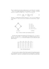Let w be a weight associated to every concept C ∈ L then, a matching measure µ is defined by weights w(C) = m({C}) ∈ [0, 1] such that µ(F1 , F2 ) = X X w(C) · C∈F1 ∩F2 !−1 w(C) C∈F2 (2) Example 1. A simple lattice with four elements: L = {C1 , C2 , C3 , C4 } defines up to five filters F = {F1 , F2 , F3 , F4 , F5 }, as shown in (a) and (b) Fig. 1, respectively. C1 F1 = {C1 } F2 = {C2 , C1 } C3 C2 F3 = {C3 , C1 } F4 = {C3 , C2 , C1 } F5 = {C4 , C3 , C2 , C1 } C4 (b) Filters (a) Lattice Fig. 1: A lattice, its filters and matching measures 1 If we give some weights to the elements of L, for instance w(C1 ) = 10 , w(C2 ) = 1 = 2 and calculate the matching measure µ(Fi , Fj ) ≤ 5) with the formula in (2), we obtain the result shown in Fig. 2. 2 3 5 , w(C3 ) = 10 , and w(C4 ) and µ(Fj , Fi ) (for 1 ≤ i, j F1 F2 F3 F4 F5 F1 1 1 5 1 4 F2 1 1 1 F3 1 4 5 1 1 8 5 8 1 2 F4 1 1 1 1 1 9 5 9 4 9 8 9 F5 1 1 1 1 1 Fig. 2: Matching Measures It is easy to note at a glance on Fig. 2 that in general, the matching measures are not symmetric. If µ(Fg , Fr ) expresses how well a given filter Fg matches a required filter Fr , then µ(Fr , Fg ) measures the excess of skills in the given filter  Fg that are not required in Fr . And clearly, µ(Fi , Fj ) = µ(Fj , Fi ) = 1, when i = j for 1 ≤ i, j ≤ 5. Example 2. Take for instance, Fr = F3 as a required profile and two given filters Fg1 = F3 and Fg2 = F4 . They are both equally and highly qualified for the requirements in Fr given their matching measures: µ(Fg1 , Fr ) = 1 and µ(Fg2 , Fr ) = 1 although, if we consider the measures µ(Fr , Fg ): 1 2 F3 matches better than F4 as C2 is not part of the required skill set. µ(Fr , Fg1 ) = 1 and µ(Fr , Fg2 ) = 3 Internal Structure of Profile Matching In a modeled selection process where there is a set of profiles P, i.e., job and applicants profiles, defined by filters in a lattice L, we denote by ϕ the conditions to be met by profiles (either job or applicants profiles) in order to be selected, then Pϕ denotes the set of profiles in P satisfying ϕ and Pr ∈ P is a required profile driving the selection by holding the conditions ϕ. Note that, when referring to matching measures from now on, we refer on matching measures as in to formula (2) that includes weighting on the elements of the lattice L, as shown in Example 1. Definition 1. For all P ∈ Pϕ and P ′ ∈ (P − Pϕ ), P is selected and P ′ is not selected if µ(P, Pr ) > µ(P ′ , Pr ) and no subset of Pϕ satisfy this property. In order to obtain the best-k matching profiles (either job or applicant profiles) we first need to query for filters representing those profiles. Consider Fr being a filter representing the required profile Pr , a requested job profile for instance. Then, consider l being a number of filters in F (Fg1 , . . . , Fgl ) representing candidates profiles matching Pr in a certain degree, satisfying ϕ such that, their matching measures are above a threshold ti ∈ [0, 1] this is, µ(Fgx , Fr ) ≥ ti for x = 1, . . . , l. Then, every Fgx represents a finite number j of profiles (Pg1 , . . . , Pgj ), candidates profiles matching Pr , where µ(Pgy , Pr ) ≥ ti for y = 1, . . . , j and j ≤ k. Note that, the relation between filters in L and the number of related profiles represented by filters is defined by a function ν : N → N where ν(x) = j Pl and x=1 ν(x) = k. Then, any Fgl+1 is not selected as the matching value µ(Fgl+1 , Fr ) < ti . As for the second part of the definition, each filter F ∈ F is uniquely determined by its minimal elements such that, we can write F = {C1 , . . . Cr }. Then, every profile represented by a filter is also uniquely determined by the elements ′′ in F . Therefore, for any profile P in a subset of Pϕ the matching value is ′′ ′′ µ(P , P ) < ti then P does not satisfy the property.  Example 3. Assume to have a job offer profile Pa and four candidates profiles {Pb , Pc , Pd , Pe } that meet the requirements in Pa . Let’s also assume that the five profiles are represented by the filters in Example 1 such that: F4 represents {Pa , Pb } F2 represents {Pc } F3 represents {Pd , Pe } then, Fr = F4 and Fg = {F2 , F3 , F4 }. If ti = 0.5, l = 3 and k = 4. In order to obtain the best l filters satisfying ϕ, we first need to know the minimum matching value representing l filters. Thus, we start by selecting any ti . If less than l solutions are found, we increase ti (ti+1 ). If more than l solutions are found, we decrease ti (ti−1 ). The search stops when the l filters satisfying µ(Fgx , Fr ) ≥ ti for x = 1, . . . , l are found. With the optimum ti , we query for the related k profiles where µ(Pg , Pr ) ≥ ti . This assumes to be given the matching measures between all filters in L and ultimately, between all profiles represented by filters. As exposed in Example 1, matching measures between filters define a matrix (Fig 2) so do matching measures between profiles although, the number of filters is assumed to be smaller than the number of profiles (l ≤ k). If we take for instance profiles Pa , Pc , Pd from example 3 we have the minimum number of profiles producing matching measures to define a matrix of profiles. Definition 2. A Matrix M is a matrix-like structure of matching measures between the minimum number of profiles that produce all possible measures. Fig. 3 shows a matrix M where columns represent the required profiles Pr and rows represent the given profiles Pg . P1 P2 ... Pn P1 µ(P1 , P1 ) µ(P1 , P2 ) . . . µ(P1 , Pn ) P2 µ(P2 , P1 ) µ(P2 , P2 ) . . . µ(P2 , Pn ) P3 .. . µ(P3 , P1 ) µ(P3 , P2 ) . . . .. .. .. . . . µ(P3 , Pn ) .. . Pn µ(Pn , P1 ) µ(Pn , P2 ) . . . µ(Pn , Pn ) Fig. 3: Matrix M of profiles Obtaining the k solutions in M involves refer either to one column or to one row. The the process is analogous if we focus either on rows or columns although, the perspective is different. While reading the measures from the columns perspective provides the so called fitness between profiles µ(Pg , Pr ), the measures  read from the rows perspective are the inverted measure µ(Pr , Pg ) denoted as overqualification. Overqualification may be considered as emphasized in Example 2 where profiles that equally (or almost equally) match the requirements, maybe subject to a second ranking with respect to the inverted measure. If we focus on columns, when querying for a particular Pr representing the required skill set, there would be finitely many profiles Pg matching Pr . Although, we only focus on the k elements where µ(Pg , Pr ) ≥ ti . Ideally, all elements in the column are in total order according to the ≤ relation of µ(Pg , Pr ). The advantage in here is that when searching for any given k and ti we only need to point to the right element in the column and search for the next consecutive k − 1 elements in descending order of matching measures. If searching for the less overqualified, there would be finitely many Pr in every row of the Matching Matrix when querying for a particular Pg but we only need to point to the right ti and search for the next k − 1 elements in ascending order of µ(Pr , Pg ). Example 4. Profiles Pa , Pc , Pd are the minimum number of profiles from Example 3 regarding fitness Pc Pd Pa - - Pd - - 5 8 1 2 Pa - - 1 Pc Fig. 4: Matching Measures We explain next how we organize profiles in order to provide an efficient search of these elements when querying for the best k-profile matching. We first assume an identification label for every row and column in Matching Matrix M, where ρi represents a number i of rows and σi represents the number i of columns, for i > 0. Definition 3. A profile record of a required profile Pr in column σi in M, is a finite number of elements < = (µi , n> i , ni , ni , next, prev, p) where µi denotes the matching measures µ(Pg , Pr ) for every matching profile Pg and n> i n= i n< i next denotes the number of profiles Pg in σi where µ(Pg , Pr ) > µi , denotes the number of profiles Pg in σi where µ(Pg , Pr ) = µi , denotes the number of profiles Pg in σi where µ(Pg , Pr ) < µi , is a reference to the next matching value in σi where µ(Pg+1 , Pr ) ≥ µi ,  prev is a reference to the next matching value in σi where µ(Pg−1 , Pr ) ≤ µi and, p is a reference to a linked-list of profiles matching Pr . < = The numbers n> i , ni , ni are significantly important when determining the number of profiles (either applicants or job profiles) represented by a filter with= out actually querying for them. It is easy to determine whether (n> i + ni ) ≥ k when querying for the pair (Pg , Pr ). Then, search for the next pair (Pg+1 , Pr ) if that is not the case. References Next and Prev make possible to track the following greater or smaller matching value of profiles by following the references. Every µi contains additionally a reference p to the related profiles (jobs or applicants) in σi column. All the related profiles are organized in a linked-list like structure of profiles, ordered by the smaller-than-or-equal elements of matching values. 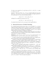Example 5. Consider the profiles {Pa , Pb , Pc , Pd , Pe } as in Example 3 with matching measures: µ(Pb , Pa ) = 1, µ(Pc , Pa ) = 0.63, µ(Pd , Pa ) = µ(Pe , Pa ) = 0.5. Consider also the graphic in Fig. 5, representing the profile records of column σi in M corresponding to Pa 0.5 Fig. 5: Linked list of matching measures Organizing data in a structure like M with profile records implies a fast and efficient search of the k matching profiles where the main objective is to fetch the < = corresponding columns σi and together with n> i ,ni and ni calculate how many of profile records we need in order to get k profiles, then follow the linked-list of profiles until the k elements are found. If we need k = 3 with ti ≥ 0.5 we could get to profile record 1 in Example 5 where there are in total 4 (2 + 2 + 0) matching profiles where: 2 profiles have matching measures ≥ 0.5, 2 profiles match Pa with = 0.5 and, none matches Pa with measures ≤ 0.5. then, we know we have to visit 2 profile records to get the total number of profiles. Of course, one can claim that starting on row 3 of Example 3 is the best  approach. Therefore, an ordering on the elements of columns in M seems to be essential. The definition of matching records on rows of Matching Matrix M is analogous to Definition 3 Definition 4. A matching record of a given profile Pg in row ρi in M, is a finite number of elements < = (µi , n> i , ni , ni , next, prev, p) where µi denotes the matching value µ(Pr , Pg ) for every matching profile Pr and n> i n= i n< i next prev p denotes the number of profiles Pr in ρi where µ(Pr , Pg ) > µi , denotes the number of profiles Pr in ρi where µ(Pr , Pg ) = µi , denotes the number of profiles Pr in ρi where µ(Pr , Pg ) < µi , is a reference to a matching values in ρi where µ(Pr+ 1 , Pg ) ≥ µi , is a reference to a matching values in ρi where µ(Pr− 1 , Pg ) ≤ µi and, is a reference to a linked-list of profiles matching Pg . The consideration regarding ordering on elements of rows in M in Definition 4 is also to be consider in order to achieve an efficient retrieval of matching overqualified profiles for a given Pg . The following section shows an implementation of the Matrix M and profile records in a relational database schema. We define the database structure supporting our definition of top-k queries in Section 3.1 while in Section 3.2 we show an algorithm that implements our definition of top-k queries in profile matching in relational databases. 3.1 Implementation of Top-K Profile Matching Our implementation approach of top-k queries as described in Section 3 is designed on a relational database schema. The schema HR shown in Fig. 6 is designed to store and maintain filters of a given lattice L, as well as profiles and matching measures of an instance of L for the implementation of top-k queries. Note that for the definition of the database schema we use the notation of the unnamed and logic programing perspective as defined in [1]. Where, under the unnamed perspective, a tuple ha1 , . . . , an i is an ordered n-tuple (n > 0) of constants of a Cartesian product domn (where dom is the underlying set of constants, the domain). As for the programming perspective, a relation R with arity n is an expression of the form R(a1 , . . . , an ) where ai ∈ dom for i ∈ [1, n] are the attributes of the relation. The database schema HR is composed by eight relation names: Filter, describes every filter in a given lattice L. If we consider the lattice L in Example 1, Filter contains 5 tuples: hF1 i, hF2 i, hF3 i, hF4 i, hF5 i. Concept describes all concepts in a Knowledge Base. An instance of Concept based on Example 1 is hC1 i, hC2 i, hC3 i, hC4 i. FilterComposition represents the relation between concepts and filters within a