ME 227 Midterm Report (PDF)
File information
This PDF 1.5 document has been generated by / Skia/PDF m71, and has been sent on pdf-archive.com on 22/10/2018 at 03:49, from IP address 69.27.x.x.
The current document download page has been viewed 231 times.
File size: 237.81 KB (5 pages).
Privacy: public file

File preview
Anna Olson | Jess Moss | Jose Juarez | Robert Kobara
18 May 2017
ME227 Midterm Report
I.
Controller Descriptions
Longitudinal Controller
We designed a simple proportional controller for our speed control. We had a feedforward term
that accounted for D’Alambert’s force, drag and rolling resistance. We developed the value
for our gain by testing different values in simulation. We tried to keep the gain as low as
possible while still matching path during simulations.
Steering Controller 1
b
a
K = mL ( Caf
- Car
)
ΔΨ ss = k(
δ FF =
δ rad =
K la xla
C af
K
- C la
af
maU x 2
LCar
- b)
2
ΔΨ ss + k(L + KU
x)
(em + Xla ΔΨ ) + δ FF
The control effort is dictated by combination proportional and feedforward controller. The
proportional term stems from the combination of the current lateral error of from the path
(em) and the lookahead error (Xla ΔΨ ). This creates a total error that is projected a distance
of Xla down the path, which is multiplied by a proportional constant.
In addition, a feedforward term (deltaFF) is added to the controller in order to account for
constant disturbances that are present with the vehicle is moving. There are two parts in the
feedforward term, the first part accounts for the steady-state heading error ( ΔΨ ss), while
the second parts accounts for the curvature of the road.
Steering Controller 2
The second controller is based off of the first with a few alterations. The first difference
is the addition of the curvature constant (Kk), which adds control effort that is proportional
to the curvature of the path. The second difference is the addition of the error constant
(Ke). This additional term adds to the feedforward terms used in the original controller.
This constant adds control effort that is solely proportional to the lateral error, but
unlike Kla, does not add control effort based on x
la. After further analysis of the controller,
it was determined that adding this constant was equivalent to increasing Kla while reducing
xla.
The value for Kk and Ke were experimentally determined via simulation with the goal of meeting
the 30cm lateral error specification. After several iterations of trial and error, we set Kk
to 0.44 and Ke to 5.
1
II.
Speed Profile
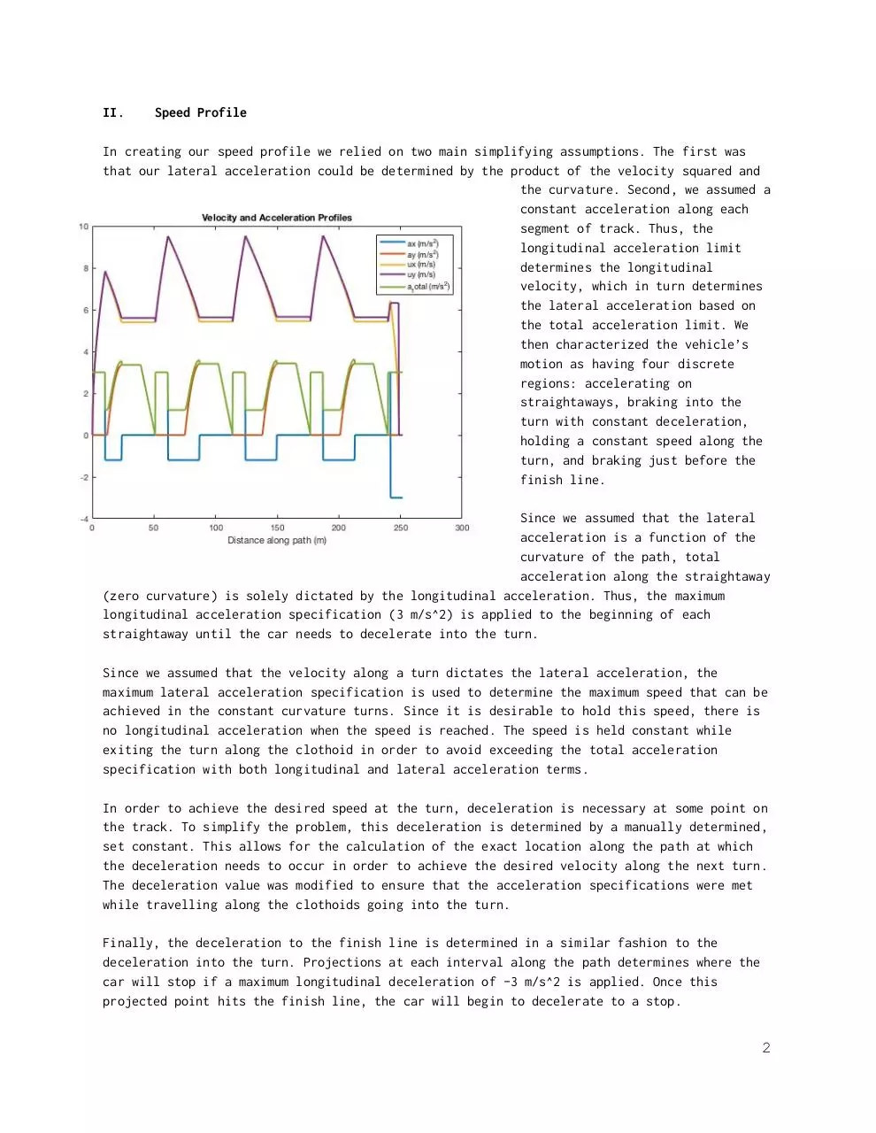
In creating our speed profile we relied on two main simplifying assumptions. The first was
that our lateral acceleration could be determined by the product of the velocity squared and
the curvature. Second, we assumed a
constant acceleration along each
segment of track. Thus, the
longitudinal acceleration limit
determines the longitudinal
velocity, which in turn determines
the lateral acceleration based on
the total acceleration limit. We
then characterized the vehicle’s
motion as having four discrete
regions: accelerating on
straightaways, braking into the
turn with constant deceleration,
holding a constant speed along the
turn, and braking just before the
finish line.
Since we assumed that the lateral
acceleration is a function of the
curvature of the path, total
acceleration along the straightaway
(zero curvature) is solely dictated by the longitudinal acceleration. Thus, the maximum
longitudinal acceleration specification (3 m/s^2) is applied to the beginning of each
straightaway until the car needs to decelerate into the turn.
Since we assumed that the velocity along a turn dictates the lateral acceleration, the
maximum lateral acceleration specification is used to determine the maximum speed that can be
achieved in the constant curvature turns. Since it is desirable to hold this speed, there is
no longitudinal acceleration when the speed is reached. The speed is held constant while
exiting the turn along the clothoid in order to avoid exceeding the total acceleration
specification with both longitudinal and lateral acceleration terms.
In order to achieve the desired speed at the turn, deceleration is necessary at some point on
the track. To simplify the problem, this deceleration is determined by a manually determined,
set constant. This allows for the calculation of the exact location along the path at which
the deceleration needs to occur in order to achieve the desired velocity along the next turn.
The deceleration value was modified to ensure that the acceleration specifications were met
while travelling along the clothoids going into the turn.
Finally, the deceleration to the finish line is determined in a similar fashion to the
deceleration into the turn. Projections at each interval along the path determines where the
car will stop if a maximum longitudinal deceleration of -3 m/s^2 is applied. Once this
projected point hits the finish line, the car will begin to decelerate to a stop.
2
III.
Experimental Results vs. Simulation
Controllers vs. Simulation
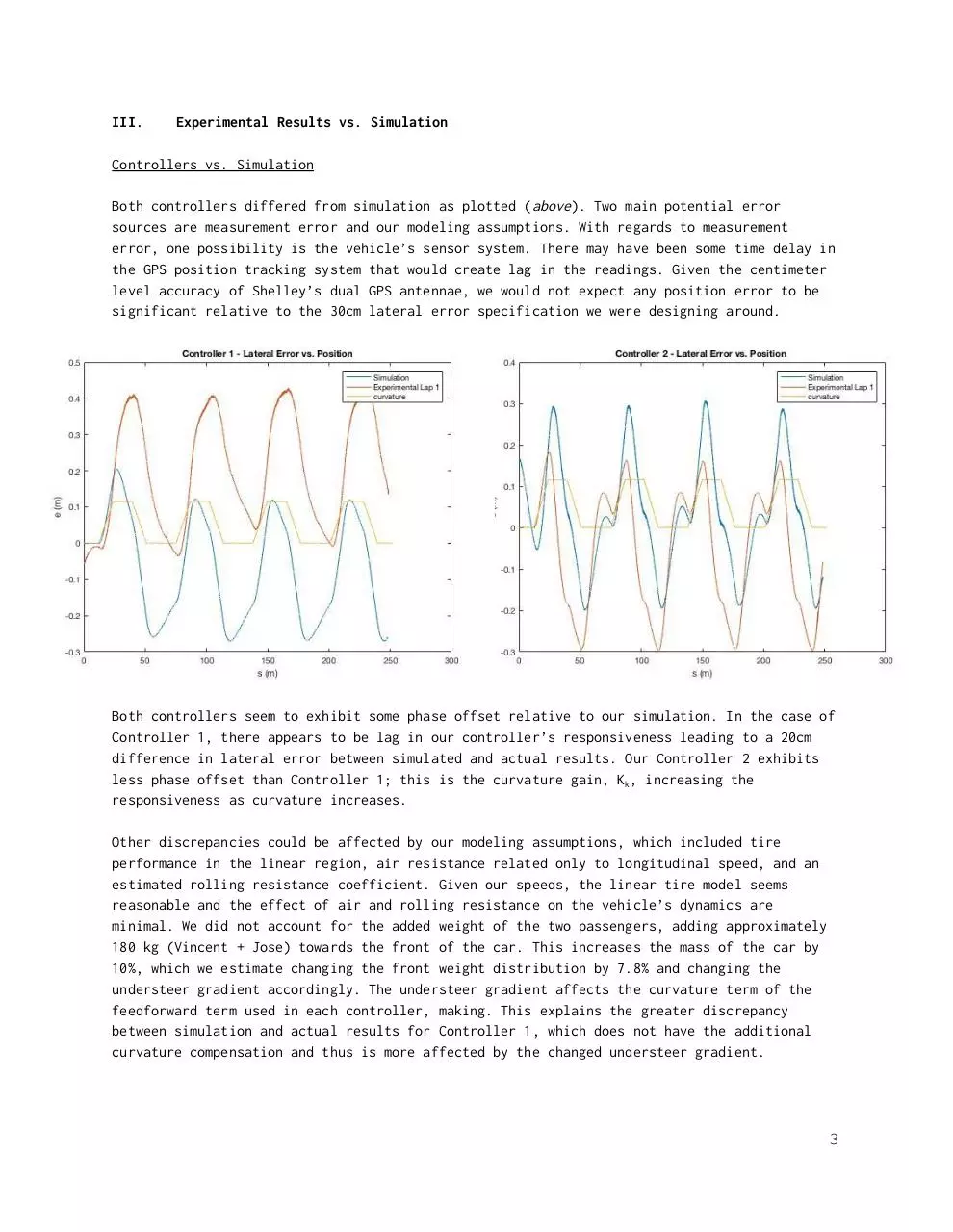
Both controllers differed from simulation as plotted (
above). Two main potential error
sources are measurement error and our modeling assumptions. With regards to measurement
error, one possibility is the vehicle’s sensor system. There may have been some time delay in
the GPS position tracking system that would create lag in the readings. Given the centimeter
level accuracy of Shelley’s dual GPS antennae, we would not expect any position error to be
significant relative to the 30cm lateral error specification we were designing around.
Both controllers seem to exhibit some phase offset relative to our simulation. In the case of
Controller 1, there appears to be lag in our controller’s responsiveness leading to a 20cm
difference in lateral error between simulated and actual results. Our Controller 2 exhibits
less phase offset than Controller 1; this is the curvature gain, K
k, increasing the
responsiveness as curvature increases.
Other discrepancies could be affected by our modeling assumptions, which included tire
performance in the linear region, air resistance related only to longitudinal speed, and an
estimated rolling resistance coefficient. Given our speeds, the linear tire model seems
reasonable and the effect of air and rolling resistance on the vehicle’s dynamics are
minimal. We did not account for the added weight of the two passengers, adding approximately
180 kg (Vincent + Jose) towards the front of the car. This increases the mass of the car by
10%, which we estimate changing the front weight distribution by 7.8% and changing the
understeer gradient accordingly. The understeer gradient affects the curvature term of the
feedforward term used in each controller, making. This explains the greater discrepancy
between simulation and actual results for Controller 1, which does not have the additional
curvature compensation and thus is more affected by the changed understeer gradient.
3
When looking at the data for the experimental and simulated data for Controller 1, the
experimental data has a much higher overshoot than the simulated data. In addition, there is
seems to be a lag in the experimental data. The discrepancy can be explained by incorrect
control effort during the turn (e.g., the passengers may be heavier or lighter than
expected). The root cause may be due to an inaccurate assumption for the weight distribution
of the car. This would lead to an inaccurate understeer ratio, which would in turn create an
inaccurate feedforward term in our controller.
Both sets of data also exhibit a vertical shift between simulated and actual results. This
difference is consistent 20cm for Controller 1 and 10cm for Controller 2. This relatively
constant difference suggests some steady state error in simulation that was unaccounted for.
Controller 1 vs. Controller 2
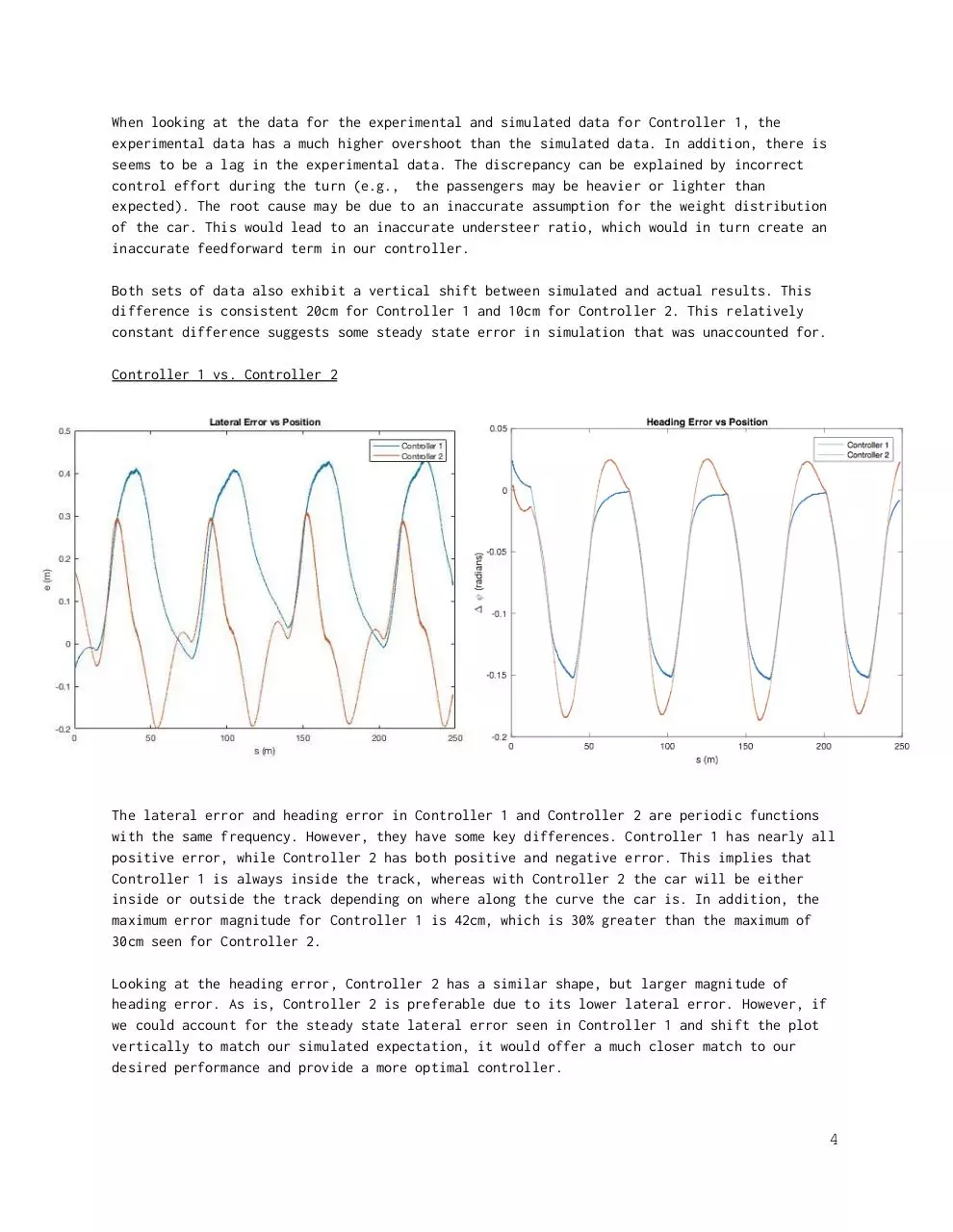
The lateral error and heading error in Controller 1 and Controller 2 are periodic functions
with the same frequency. However, they have some key differences. Controller 1 has nearly all
positive error, while Controller 2 has both positive and negative error. This implies that
Controller 1 is always inside the track, whereas with Controller 2 the car will be either
inside or outside the track depending on where along the curve the car is. In addition, the
maximum error magnitude for Controller 1 is 42cm, which is 30% greater than the maximum of
30cm seen for Controller 2.
Looking at the heading error, Controller 2 has a similar shape, but larger magnitude of
heading error. As is, Controller 2 is preferable due to its lower lateral error. However, if
we could account for the steady state lateral error seen in Controller 1 and shift the plot
vertically to match our simulated expectation, it would offer a much closer match to our
desired performance and provide a more optimal controller.
4
IV.
Conclusion
All models are wrong, some are useful.
5
Download ME 227 Midterm Report
ME 227 Midterm Report.pdf (PDF, 237.81 KB)
Download PDF
Share this file on social networks
Link to this page
Permanent link
Use the permanent link to the download page to share your document on Facebook, Twitter, LinkedIn, or directly with a contact by e-Mail, Messenger, Whatsapp, Line..
Short link
Use the short link to share your document on Twitter or by text message (SMS)
HTML Code
Copy the following HTML code to share your document on a Website or Blog
QR Code to this page

This file has been shared publicly by a user of PDF Archive.
Document ID: 0001899698.